SSH variability

Description

The sshVariability diagnostic is a part of AQUA framework’s frontier diagnostic. It calculates the sea surface height (SSH) standard deviation for models (e.g. FESOM, ICON, NEMO) and compares them against the AVISO model. This diagnotic can work on Healpix and standard Lat-Lon grid data. It also provides visualization of the SSH variability for the models. SSH variability provides insights into the complex dynamics of the ocean. It represents the changes in sea surface height over time, which can be influenced by various factors such as ocean currents, wind patterns, tides, and interactions with the atmosphere. By studying SSH variability, we can gain a better understanding of oceanic processes and their impact on climate. High-resolution climate models simulate fine-scale variations in SSH, capturing small-scale features and regional differences highly relevant in the context of climate adaptation for instance, coastal management such as managing coastal hazards like flooding or storm surges.

Classes

There are two main classes in this diagnotic namely, sshVariabilityCompute and sshVariabilityPlot.

• sshVariabilityCompute: class to compute the ssh variability. It retrieves the data on it original grid with an option of regridding the data on a different resolution. Then the ssh standard deviation (point-wise) is computed along the given time interval. If on time interval is provided, standard deviation will be perfromed over the whole domain. Then the data is stored in a netcdf file using the AQUA OutputSaver class.

• sshVariabilityPlot: class to plot the sshVariability. Once the standard deviation is performed, it can be passed to this class for plotting. This class plots the standard deviation for the given model and the reference AVISO data. It can also plot the difference between AVISO and the model standard deviation. This class also provides a functionality to plot selected region and the difference plots of the region. The user may as well choose the resoution on which they would like to plot the data.

• BaseMixin: this class is called inside the sshVariabilityCompute class. This class basically retrieves the data using the Reader class in AQUA core and provides the functionality to save the output as netcdf file.

• PlotBaseMixin: this class is called inside the sshVariabilityPlot class. It mainly provides the functionality to save the plots as PNG and PDF.

File Structure

• The diagnostic is located in src/aqua_diagnostics/sshVariability directory, which contains both the source code and the command line interface (CLI) script.

• The configuration file for the CLI is located in config/diagnostics/sshVariability directory with default options.

• A notebook is avaliable in the notebooks/diagnostics/sshVariability/sshVariability.ipynb directory with an example for using this diagnostic.

• README.md : a readme file which contains technical information on how to install the SSH diagnostic and its environment and, the version of the diagnostic.

Input variables and datasets

By default, the diagnostic compares against the AVISO dataset but can be configured to use any other dataset as a reference. zos or avg_zos is the variable which is used in this diagnostic. The output (netcdf, PNG and PDF) is stored using the OutputSaver class in both BaseMixin and PlotBaseMixin classes.

The diagnostic is designed to work with both the data from the Low Resolution Archive (LRA) and the original high resolution Healpix data. The LRA is generated by the Data reduction OPerator (DROP) of the AQUA project, which provides monthly data at a 1x1 degree resolution.

Basic Usage

The basic usage of this diagnostic is explained with a working example in the notebook provided in the notebooks/diagnostics/sshVariability directory. The basic structure of the analysis is the following:

Example usage

from aqua.diagnostics import sshVariabilityCompute, sshVariabilityPlot

# You can name these dictionaries as you like
dataset_dict = {
    "catalog": "climatedt-phase1",
    "model": "IFS-NEMO",
    "exp": "historical-1990",
    "source": "ssh-IFS-NEMO-test",
    "regrid": "r025",
}

dataset_dict_ref = {
    "catalog": "obs",
    "model": "AVISO",
    "exp": "ssh-L4",
    "source": "ssh-AVISO-test",
    "regrid": "r025",
}

startdate = "1994-01-01"
enddate = "1994-01-04"

# Initialize the SSH compute class
ssh_dataset = sshVariabilityCompute(
    **dataset_dict,
    var="zos",
    startdate=startdate,
    enddate=enddate,
)

# Run the compute function and save as NetCDF
ssh_dataset.run()

# Initialize the SSH compute class for reference data (AVISO)
ssh_dataset_ref = sshVariabilityCompute(
    **dataset_dict_ref,
    var="zos",
    startdate=startdate,
    enddate=enddate,
)

# Run the compute function and save as NetCDF
ssh_dataset_ref.run()

# Initialize the SSH plot class
plot_class = sshVariabilityPlot()

# Plot SSH for model dataset
plot_dataset = {"catalog": "climatedt-phase1", "model": "IFS-NEMO", "exp": "historical-1990"}
plot_class.plot(
    dataset_std=ssh_dataset.data_std,
    **plot_dataset,
    startdate=startdate,
    enddate=enddate,
)

# Plot SSH for reference dataset
plot_dataset_ref = {"catalog": "obs", "model": "AVISO", "exp": "ssh-L4"}
plot_class.plot(
    dataset_std=ssh_dataset_ref.data_std,
    **plot_dataset_ref,
    startdate=startdate,
    enddate=enddate,
)

# Plot the diference of sub region for model dataset and reference dataset AVISO
time_intervals = {
    "startdate": "1994-01-01",
    "enddate": "1994-01-04",
    "startdate_ref": "1994-01-01",
    "enddate_ref": "1994-01-04",
}

region_selection = {
    "region": "Agulhas",
    "lon_limits": [5, 50],
    "lat_limits": [-10, -50],
    "proj": "plate_carree",
    "proj_params": {},
    "tgt_grid_name": "r3600x1800"
}

_dataset_ref = {
    "catalog_ref": "obs",
    "model_ref": "AVISO",
    "exp_ref":"ssh-L4",
}

_dataset = {
    "catalog": "climatedt-phase1",
    "model": "IFS-NEMO",
    "exp":"historical-1990",
}

plot_class.plot_diff(
    dataset_std=ssh_dataset.data_std,
    dataset_std_ref=ssh_dataset_ref.data_std,
    **_dataset,
    **_dataset_ref,
    **region_selection,
    **time_intervals
)

Note

The user can also define the start and end date of the analysis and the reference dataset. If not specified otherwise, plots will be saved in PNG and PDF format in the current working directory.

CLI usage

The diagnostic can be run from the command line interface (CLI) by running the following command:

cd $AQUA/src/aqua_diagnostics/sshVariability
python cli_sshVariability.py --config_file <path_to_config_file>

Additionally, the CLI can be run with the following optional arguments:

• --config, -c: Path to the configuration file.

• --nworkers, -n: Number of workers to use for parallel processing.

• --cluster: Cluster to use for parallel processing. By default a local cluster is used.

• --loglevel, -l: Logging level. Default is WARNING.

• --catalog: Catalog to use for the analysis. Can be defined in the config file.

• --model: Model to analyse. Can be defined in the config file.

• --exp: Experiment to analyse. Can be defined in the config file.

• --source: Source to analyse. Can be defined in the config file.

• --outputdir: Output directory for the plots.

Config file structure

The configuration file is a YAML file that contains the details on the dataset to analyse or use as reference, the output directory and the diagnostic settings. Most of the settings are common to all the diagnostics (see Diagnostics configuration files). Here we describe only the specific settings for the sshVariability diagnostic.

• sshVariability: a block (nested in the diagnostics block) containing options for the SSH Variability diagnostic. Variable-specific parameters override the defaults.

  • run: enable/disable the diagnostic.

  • diagnostic_name: name of the diagnostic. sshVariability by default.

  • variables: list of variables to analyse. In sshVariability this variable is zos or avg_zos.

  • startdate_data / enddate_data: time range for the dataset.

  • startdate_ref / enddate_ref: time range for the reference dataset.

diagnostics:
    sshVariability:
    run: true
    diagnostic_name: 'sshVariability'
    variables: 'zos'
    params:
        default:
            startdate_data: '1994-01-01'
            enddate_data: '1994-01-04'
            startdate_ref: '1994-01-01'
            enddate_ref: '1994-01-04'

• plot_params: defines colorbar palette and limits and projection parameters. The default parameters are used if not specified. Refer to ‘src/aqua/util/projections.py’ for available projections. Note that the plots can be stored on the original resolution or the data can be regridded to another resolution for a quick plot. The default for plotting regrid variable tgt_grid_name: 'r360x180' with the regridding method regrid_method: 'ycon'. More options for regridding are documented on the topic of Regridding in AQUA <https://aqua.readthedocs.io/en/latest/regrid.html>_

plot_params:
    default:
        projection: 'robinson'
        projection_params: {}
        vmin:
        vmax:
        cmap: 'RdBu_r'
        tgt_grid_name: 'r360x180'
        regrid_method: 'ycon'
    # sub region selection
    sub_region :
        name: Agulhas
        lon_limits: [5, 50]
        lat_limits: [-10, -50]
        projection: 'plate_carree'
        projection_params: {}
    # ONLY FOR ICON: Flags for northern and southern boundaries to mask out specific latitudes.
    # As AVISO does not have data under the sea ice, which ICON does,
    # to make the datasets comparable - SSH under sea ice for ICON can be masked out.
    mask_options:
        mask_northern_boundary: true
        mask_southern_boundary: true
        northern_boundary_latitude: 70
        southern_boundary_latitude: -62

Output

The diagnostic produces four types of plots:

• Global SSH variability plots for the given model and the reference.

• Global difference plot (model vs reference)

• Regional SSH variability plots for the given model and the reference.

• Regional difference plot (model vs reference)

Plots are saved in both PDF and PNG format.

Observations

The default reference dataset is from AVISO Sea Surface Height Data, but custom references can be configured.

References

• Copernicus Climate Change Service, Climate Data Store, (2018): Sea level gridded data from satellite observations for the global ocean from 1993 to present. Copernicus Climate Change Service (C3S) Climate Data Store (CDS). DOI: 10.24381/cds.4c328c78 (Accessed on 01-Mar-2023)

Example Plot(s)

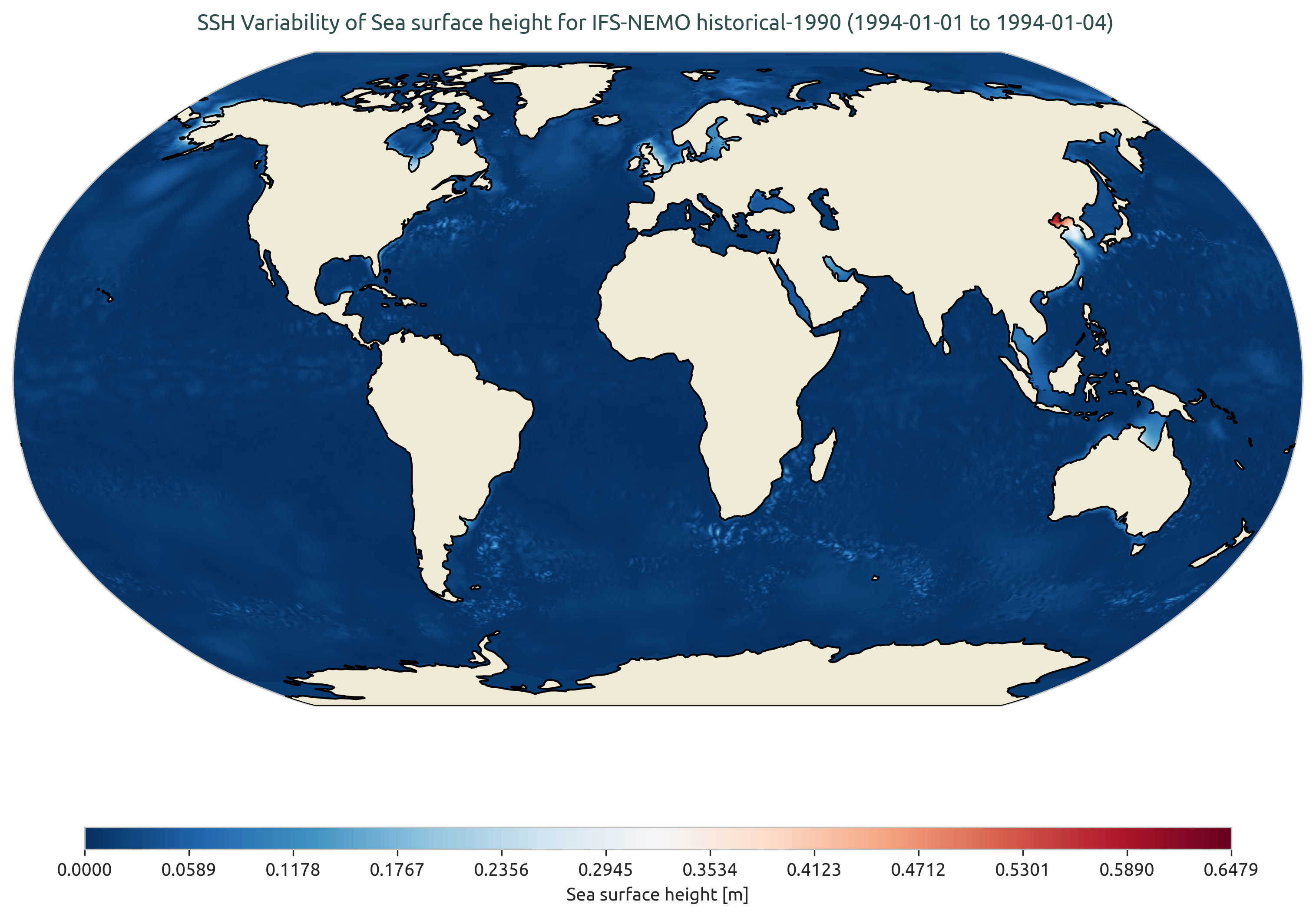
SSH Variability for IFS-NEMO historical-1990.

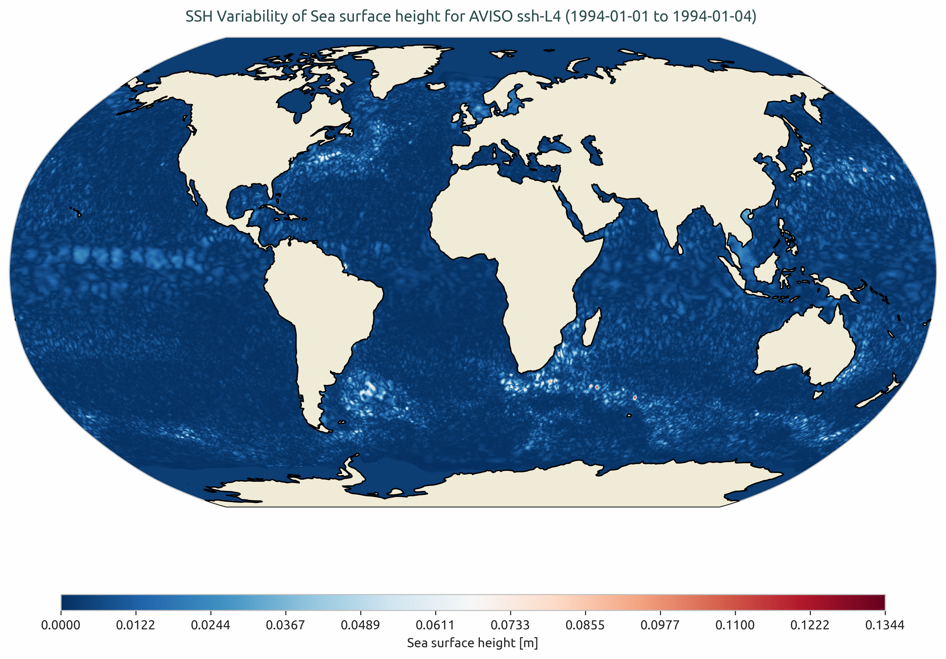
SSH Variability for AVISO data.

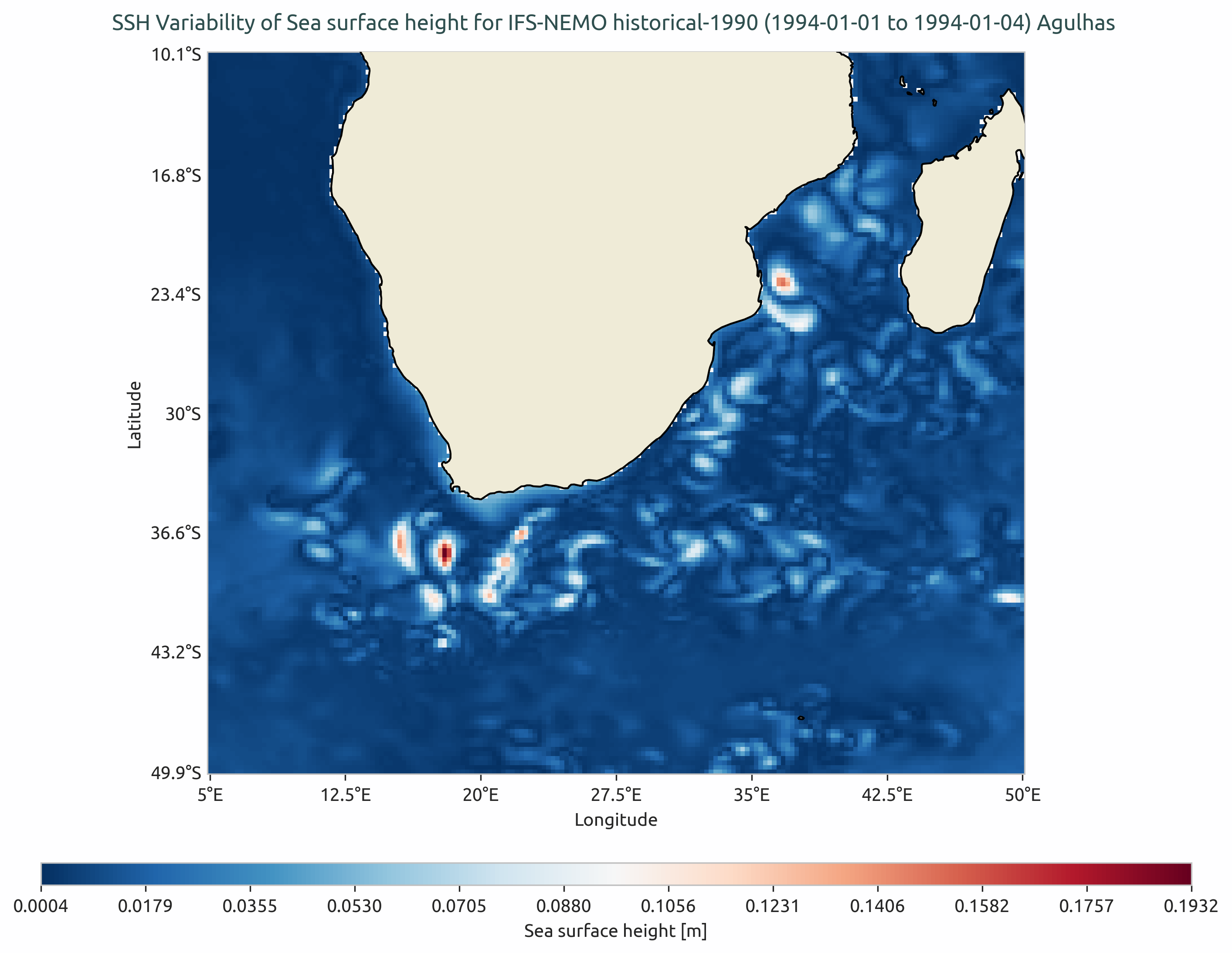
SSH Variability for IFS-NEMO in Agulhas region.

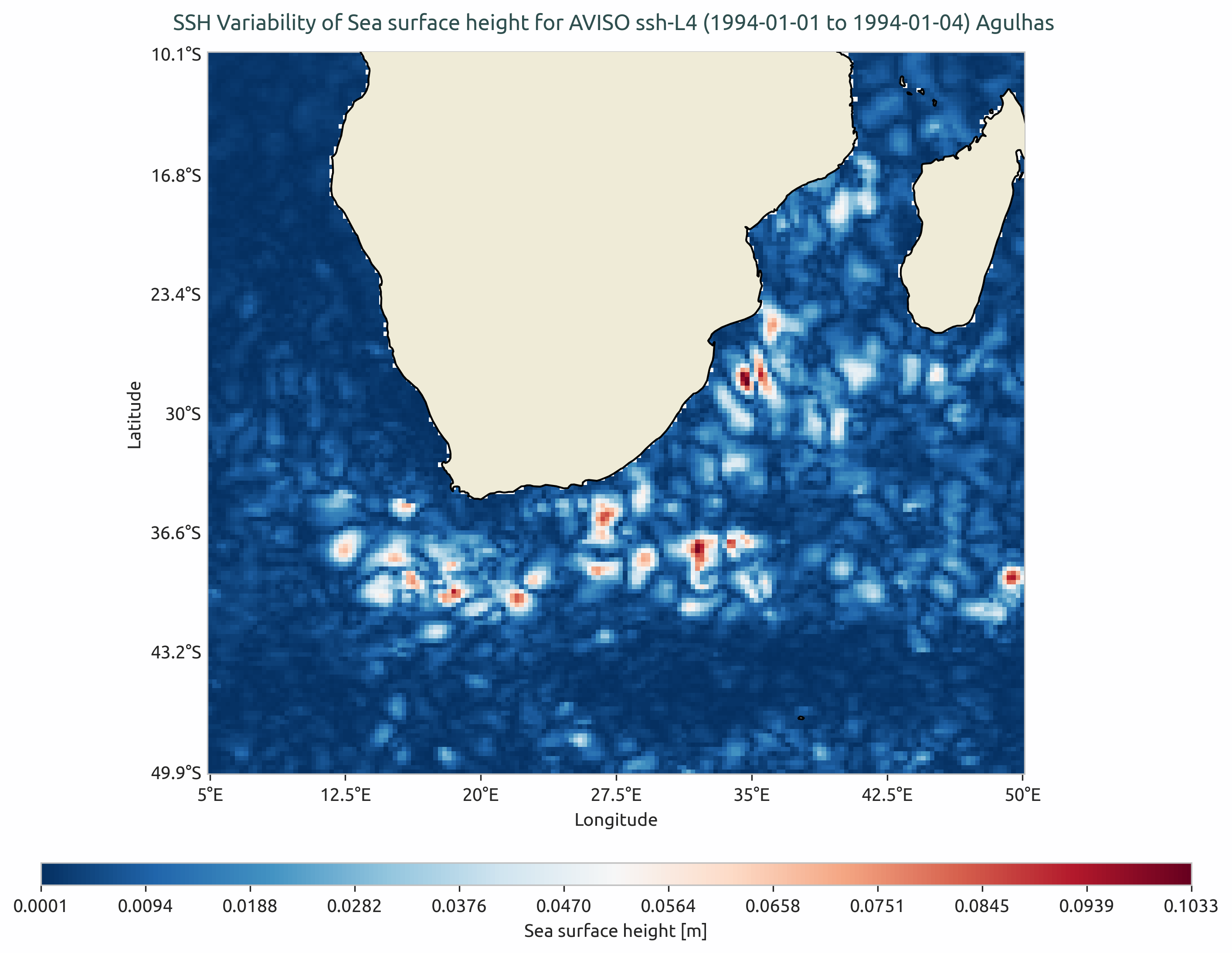
SSH Variability for AVISO in Agulhas region.

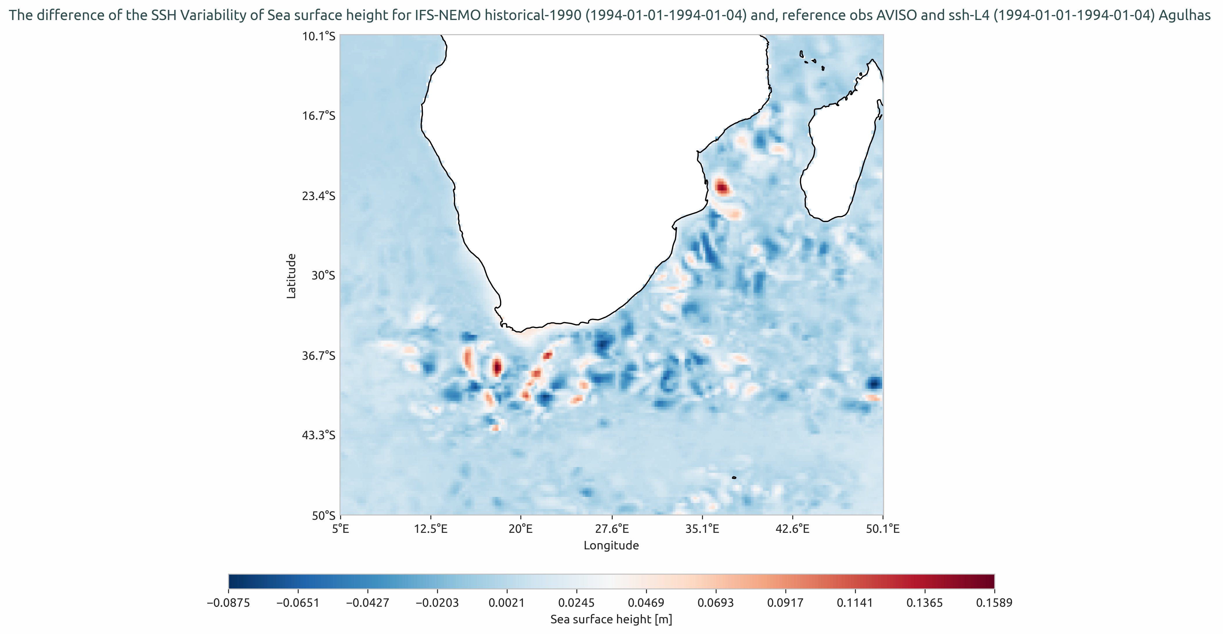
SSH Variability difference between IFS-NEMO and AVISO in Agulhas region.

Available demo notebooks

Notebooks are stored in the notebooks/diagnostics/sshVariability directory and contain usage examples.

• sshVariability.ipynb

Authors and contributors

This diagnostic is authored and maintained by Maqsood Mubarak Rajput (@maqsoodrajput, maqsoodmubarak.rajput@awi.de). Contributions are welcome — please open an issue or a pull request. For questions or suggestions, contact the AQUA team or the maintainers.

Detailed API

This section provides a detailed reference for the Application Programming Interface (API) of the sshVariability diagnostic, produced from the diagnostic function docstrings.

ssh module

class aqua.diagnostics.sshVariability.sshVariabilityCompute(diagnostic_name: str = 'sshVariability', catalog: str = None, model: str = None, exp: str = None, source: str = None, startdate: str = None, enddate: str = None, freq: str = None, region: str = None, regrid: str = None, lon_limits: list[float] = None, lat_limits: list[float] = None, var: str = 'zos', long_name: str = None, short_name: str = None, units: str = None, save_netcdf: bool = True, rebuild: bool = True, outputdir: str = './', reader_kwargs: dict = {}, loglevel: str = 'WARNING')

Bases: BaseMixin

SSH Computation

Initialize the ‘sshVariabilityCompute’ class.

This class is designed to load an xarray.Dataset and computes STD. :param diagnostic_name: Default is ‘sshVariability’. :type diagnostic_name: str :param catalog: catalog. It is Mandatory, if ‘save_netcdf=True’. :type catalog: str :param model: Name of the data :type model: str :param exp: Name of the experiment :type exp: str :param source: the source. :type source: str :param It is important to give these dates and input. Otherwise the whole dataset is retrieved.: :param startdate: Start date. :type startdate: str :param enddate: End date. :type enddate: str :param freq: Frequency of the data. In the TODO list. This becomes important when implementing the ‘variance of the variances formula’. :type freq: str :param region: For subregion selection. Default is ‘None’. In case of sub-region STD computation, this variable is mandatory. :type region: str :param regrid: Regrid option for the data. NOTE: the regridding will be applied before computing the STD. :type regrid: str :param If ‘lon_limits’ and ‘lat_limits’ are None: :param they are taken from region file in AQUA.: :param lon_limits: list of lon limits. Default is ‘None’. :type lon_limits: list[float] :param lat_limits: list of lat limits. Default is ‘None’. :type lat_limits: list[float] :param var: Variable name for ssh data. Default is ‘zos’. :type var: str :param long_name: If not given extracted from the data. :type long_name: str :param short_name: If not given extracted from the data. :type short_name: str :param units: If not given extracted from the data. :type units: str :param save_netcdf: Default is ‘True’. :type save_netcdf: bool :param rebuild: Recomputes and saves the netcdf. Default is “True”. :type rebuild: bool :param outputdir: output directory. Default is ‘./’ :type outputdir: str :param loglevel: Default WARNING. :type loglevel: str

Keyword Arguments:

• zoom (int, optional) – HEALPix grid zoom level (e.g. zoom=10 is h1024). Allows for multiple gridname definitions.

• realization (int, optional) – The ensemble realization number, included in the output filename.

• **kwargs – Additional arbitrary keyword arguments to be passed as additional parameters to the intake catalog entry.

run()

Parameters:

create_catalog_entry (bool) – Option for creating catalog entry. Default is ‘False’.

This function performs following three functions: a) Retrieve data and regrid if given then b) Compute STD c) Save netcdf