Ocean Stratification Diagnostic

Description

The OceanStratification diagnostic is a set of tools for the analysis and visualization of ocean stratification and mixed layer depth (MLD) in climate model outputs. It supports comparative analysis between a target dataset (typically a climate model) and a reference, commonly an observational dataset such as EN4.

Ocean Stratification provides tools to:

Compute potential density from temperature and salinity fields
Calculate mixed layer depth (MLD)
Generate vertical stratification profiles averaged over specific basins
Produce climatological analyses (monthly, seasonal, yearly, or total period)

Classes

The diagnostic is designed with a class that analyzes ocean data and computes stratification metrics, and other two classes that produces the plots.

Stratification: retrieves ocean data (temperature, salinity) and computes derived quantities including potential density and mixed layer depth. It handles spatial averaging over specified regions, climatology computation, and unit conversions. Results are saved as class attributes and as NetCDF files.
PlotStratification: provides methods for plotting vertical stratification profiles of temperature, salinity, and density. It generates multi-panel plots comparing model and reference data across different variables.
PlotMLD: specialized class for plotting mixed layer depth maps and statistics. It generates spatial maps and comparative visualizations of MLD fields.

File structure

The diagnostic is located in the aqua/diagnostics/ocean_stratification directory, which contains both the source code and the command line interface (CLI) script.
A template configuration file is available at aqua/diagnostics/templates/diagnostics/config-stratification.yaml
Notebooks are available in the notebooks/diagnostics/ocean_stratification directory and contain examples of how to use the diagnostic.
Regions definitions are available in aqua/diagnostics/config/tools/ocean3d/definitions/regions.yaml

Input variables and datasets

By default, the diagnostic compares against the EN4 dataset, but it can be configured to use any other dataset as a reference. The diagnostic requires 3D ocean data that includes vertical level information (depth or pressure).

The primary variables used in this diagnostic are:

thetao (sea water potential temperature)
so (sea water salinity)

Derived variables computed by the diagnostic:

rho (potential density anomaly)
mld (mixed layer depth)

The diagnostic is designed to work with data from the Low Resolution Archive (LRA), generated by the Data reduction OPerator (DROP) of the AQUA project, which provides monthly data at a 1x1 degree resolution. A higher resolution is not necessary for this diagnostic.

Basic usage

The basic usage of this diagnostic is explained with a working example in the notebook. The basic structure of the analysis is the following:

from aqua.diagnostics import Stratification, PlotStratification, PlotMLD

strat = Stratification(
    catalog='climatedt-phase1',
    model='IFS-NEMO',
    exp='historical-1990',
    source='lra-r100-monthly',
    startdate='01-01-1991',
    enddate='31-05-1992',
    loglevel='DEBUG'
)

strat.run(
    dim_mean=["lat","lon"],
    outputdir=".",
    var=['thetao', 'so'],
    region="ls",
    mld=False,
    climatology="January",
)

ps = PlotStratification(
    data=strat.data[['thetao', 'so', 'rho']],
    obs=strat.data[['thetao', 'so', 'rho']]*1.001,  # just to have different data for obs
    loglevel='DEBUG',
)
ps.plot_stratification()

ps = PlotMLD(
    data=strat.data[['mld']],
    obs=strat.data[['mld']]*1.1,
    loglevel='DEBUG',
)
ps.plot_mld()

CLI usage

The diagnostic can be run from the command line interface (CLI) by running the following command:

cd $AQUA/aqua/diagnostics/ocean_stratification
python cli_ocean_stratification.py --config <path_to_config_file>

Additionally, the CLI can be run with the following optional arguments:

--config, -c: Path to the configuration file.
--nworkers, -n: Number of workers to use for parallel processing.
--cluster: Cluster to use for parallel processing. By default a local cluster is used.
--loglevel, -l: Logging level. Default is WARNING.
--catalog: Catalog to use for the analysis. Can be defined in the config file.
--model: Model to analyse. Can be defined in the config file.
--exp: Experiment to analyse. Can be defined in the config file.
--source: Source to analyse. Can be defined in the config file.
--outputdir: Output directory for the plots.
--startdate: Start date for the analysis.
--enddate: End date for the analysis.

Configuration file structure

The configuration file is a YAML file that contains the details on the dataset to analyse or use as reference, the output directory and the diagnostic settings. Most of the settings are common to all the diagnostics (see Diagnostics configuration files). Here we describe only the specific settings for the ocean stratification diagnostic.

ocean_stratification: a block (nested in the diagnostics block) containing options for the Ocean Stratification diagnostic.
- stratification: sub-block containing specific parameters for stratification analysis.
  - run: enable/disable the diagnostic.
  - diagnostic_name: name of the diagnostic. ocean3d by default.
  - vert_coord: vertical coordinate for the analysis (e.g., level).
  - var: list of variables to analyse (typically ['thetao', 'so']).
  - regions: list of ocean regions to analyse (e.g., ['ls', 'is', 'ws', 'gs', 'ros']).
  - climatology: list of climatology periods corresponding to each region (e.g., ['DJF', 'JJA', 'JJA', 'DJF', 'DJF']).
  - dim_mean: dimensions over which to compute spatial averages (typically ['lat', 'lon']).

Note

The regions and climatology parameters are zipped together, so if you want the same region with different climatologies, you need to repeat the region name.

diagnostics:
  ocean_stratification:
    stratification:
      diagnostic_name: 'ocean3d'
      vert_coord: level
      run: true
      var: ['thetao', 'so']
      regions: ['ls', 'is', 'ws', 'gs', 'ros']
      climatology: ['DJF', 'JJA', 'JJA', 'DJF', 'DJF']

The diagnostic supports analysis over predefined ocean regions. Common regions include:

ls - Labrador Sea
is - Irminger Sea
ws - Weddell Sea
gs - Greenland Sea
ros - Ross Sea
global - Global ocean (default if no region specified)

Additional regions can be defined in aqua/diagnostics/config/tools/ocean3d/definitions/regions.yaml.

Output

The diagnostic produces two types of plots:

Vertical stratification profiles showing temperature, salinity, and density as functions of depth
Multi-panel Mixed Layer Depth spatial maps

Plots are saved in both PDF and PNG format. Data outputs (containing rho, mld and original variables computed over the specified regions) are saved as NetCDF files for further analysis.

Observations

The default reference dataset is EN4.2.2.g10 (from 1950 to 2022), but custom references can be specified in the configuration file.

References

Potential density calculation is based on polyTEOS-10 see: https://github.com/fabien-roquet/polyTEOS/blob/36b9aef6cd2755823b5d3a7349cfe64a6823a73e/polyTEOS10.py#L57
de Boyer Montégut, C., Madec, G., Fischer, A. S., Lazar, A., and Iudicone, D. (2004): Mixed layer depth over the global ocean: An examination of profile data and a profile-based climatology. J. Geophys. Res., 109, C12003, doi:10.1029/2004JC002378
Gouretski and Reseghetti (2010): On depth and temperature biases in bathythermograph data: development of a new correction scheme based on analysis of a global ocean database. Deep-Sea Research I, 57, 6. doi: http://dx.doi.org/10.1016/j.dsr.2010.03.011
https://www.teos-10.org/

Example Plots

All plots can be reproduced using the notebooks in the notebooks directory on LUMI HPC.

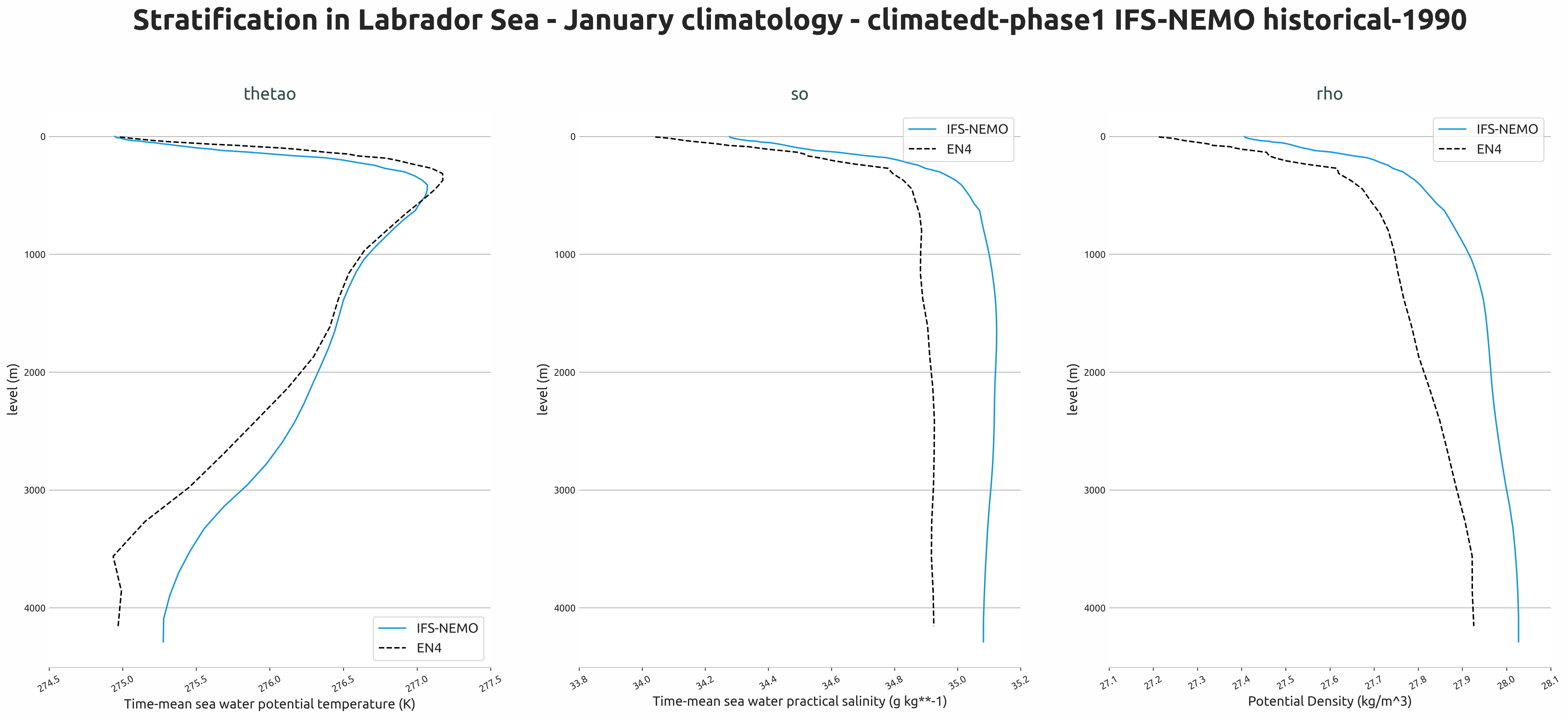
../_images/ocean_stratification.stratification.climatedt-phase1.IFS-NEMO.historical-1990.r1.labrador_sea.png — Vertical stratification profiles of temperature, salinity, and density in the Labrador Sea (January climatology) from IFS-NEMO historical-1990 experiment compared to EN4 observations.

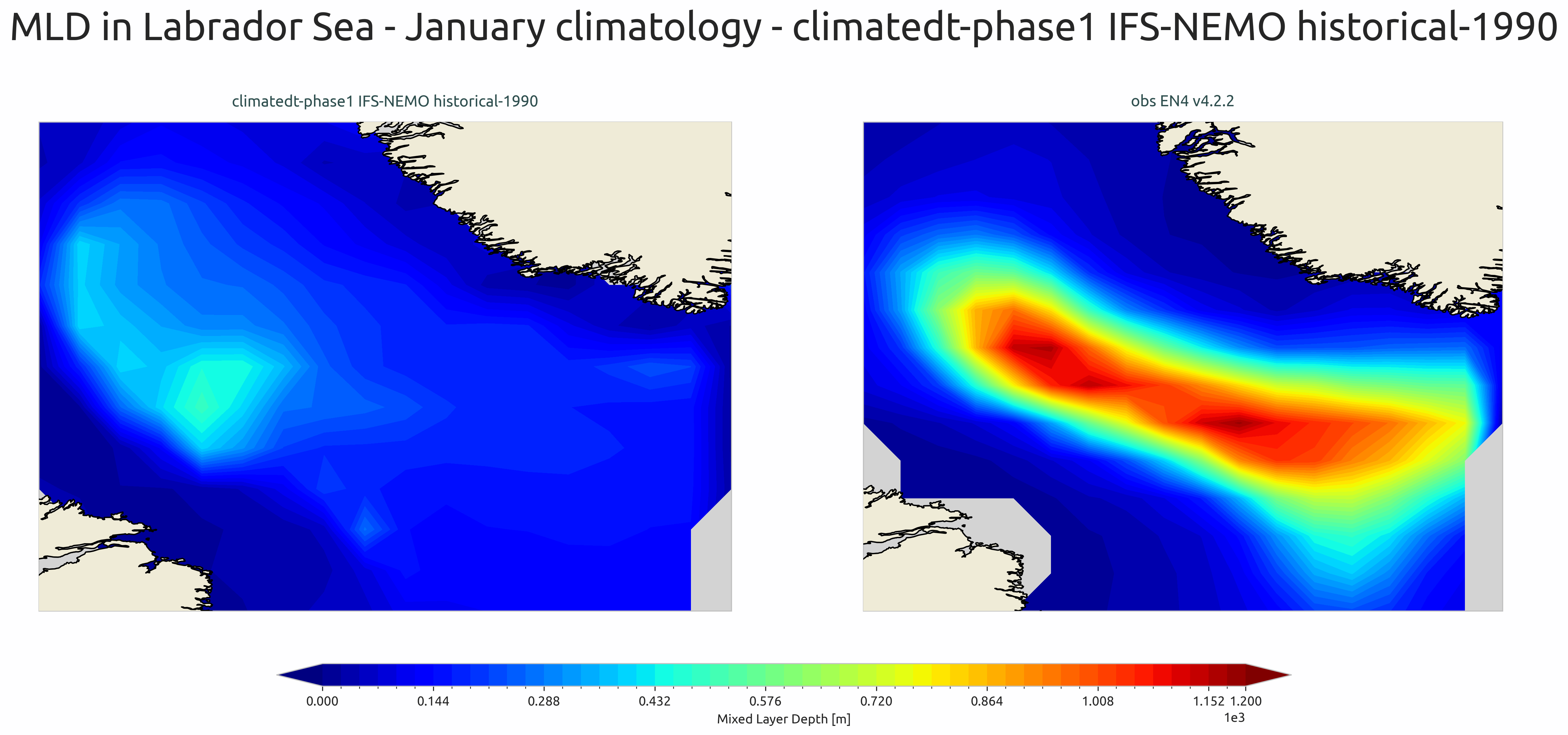
../_images/ocean_stratification.mld.climatedt-phase1.IFS-NEMO.historical-1990.r1.labrador_sea.png — Mixed layer depth spatial distribution for January climatology in the Labrador Sea from IFS-NEMO historical-1990 experiment compared to EN4 observations.

Available demo notebooks

Notebooks are stored in notebooks/diagnostics/ocean_stratification:

stratification.ipynb

Authors and contributors

This diagnostic is maintained by Supriyo Gosh (@ghossh, supriyo.ghosh@bsc.es). Contributions are welcome — please open an issue or a pull request. For questions or suggestions, contact the AQUA team or the maintainer.

Detailed API

This section provides a detailed reference for the Application Programming Interface (API) of the “ocean3d” diagnostic, produced from the diagnostic function docstrings.

class aqua.diagnostics.ocean_stratification.PlotMLD(data: Dataset, obs: Dataset = None, diagnostic_name: str = 'ocean_stratification', outputdir: str = '.', loglevel: str = 'WARNING')

Bases: object

Class to plot Mixed Layer Depth (MLD) maps.

Parameters:

data (xr.Dataset) – Dataset containing the MLD data to be plotted.
obs (xr.Dataset, optional) – Dataset containing observational MLD data for comparison. Default is None.
clim_time (str, optional) – Climatological time period for the data. Default is “January”.
diagnostic_name (str, optional) – Name of the diagnostic. Default is “ocean_stratification”.
outputdir (str, optional) – Directory to save the output plots. Default is the current directory.
loglevel (str, optional) – Logging level. Default is “WARNING”.

plot_mld(rebuild: bool = True, save_pdf: bool = True, save_png: bool = True, dpi: int = 300)

save_plot(fig, diagnostic_product: str = None, extra_keys: dict = None, rebuild: bool = True, dpi: int = 300, format: str = 'png', metadata: dict = None)

Save the plot to a file.

Parameters:

fig (matplotlib.figure.Figure) – The figure to be saved.
diagnostic_product (str) – The name of the diagnostic product. Default is None.
extra_keys (dict) – Extra keys to be used for the filename (e.g. season). Default is None.
rebuild (bool) – If True, the output files will be rebuilt. Default is True.
dpi (int) – The dpi of the figure. Default is 300.
format (str) – The format of the figure. Default is ‘png’.
metadata (dict) – The metadata to be used for the figure. Default is None. They will be complemented with the metadata from the outputsaver. We usually want to add here the description of the figure.

set_cbar_labels(var: str = None)

set_cbar_limits()

set_central_longitude()

set_convert_lon(data=None): Convert longitude from 0-360 to -180 to 180 and sort accordingly.

set_data_map_list()

set_description()

set_figsize()

set_nrowcol()

set_suptitle(plot_type=None): Set the title for the MLD plot.

set_title(): Set the title for the Hovmoller plot. This method can be extended to set specific titles based on the data.

set_ytext()

class aqua.diagnostics.ocean_stratification.PlotStratification(data: Dataset, obs: Dataset = None, diagnostic_name: str = 'ocean_stratification', vert_coord: str = 'level', outputdir: str = '.', loglevel: str = 'WARNING')

Bases: object

plot_stratification(rebuild: bool = True, save_pdf: bool = True, save_png: bool = True, dpi: int = 300)

save_plot(fig, diagnostic_product: str = None, extra_keys: dict = None, rebuild: bool = True, dpi: int = 300, format: str = 'png', metadata: dict = None)

Save the plot to a file.

Parameters:

fig (matplotlib.figure.Figure) – The figure to be saved.
diagnostic_product (str) – The name of the diagnostic product. Default is None.
extra_keys (dict) – Extra keys to be used for the filename (e.g. season). Default is None.
rebuild (bool) – If True, the output files will be rebuilt. Default is True.
dpi (int) – The dpi of the figure. Default is 300.
format (str) – The format of the figure. Default is ‘png’.
metadata (dict) – The metadata to be used for the figure. Default is None. They will be complemented with the metadata from the outputsaver. We usually want to add here the description of the figure.

set_cbar_labels(var: str = None)

set_cbar_limits()

set_data_list()

set_description()

set_label_line_plot()

set_nrowcol()

set_suptitle(plot_type=None): Set the title for the MLD plot.

set_title(): Set the title for the Hovmoller plot. This method can be extended to set specific titles based on the data.

set_ytext()

class aqua.diagnostics.ocean_stratification.Stratification(catalog: str = None, model: str = None, exp: str = None, source: str = None, regrid: str = None, startdate: str = None, enddate: str = None, diagnostic_name: str = 'stratification', vert_coord: str = 'level', loglevel: str = 'WARNING')

Bases: Diagnostic

Diagnostic class for analyzing ocean stratification.

Parameters

catalogstr, optional: Path to the data catalog (e.g., intake-esm catalog).
modelstr, optional: Name of the climate model to analyze.
expstr, optional: Experiment name (e.g., ‘historical’, ‘ssp585’).
sourcestr, optional: Data source (e.g., ‘CMIP6’, ‘OBS’).
regridstr, optional: Regridding method or target grid (e.g., ‘1x1’, ‘nearest’).
startdatestr, optional: Start date of the analysis period (format: ‘YYYY-MM-DD’).
enddatestr, optional: End date of the analysis period (format: ‘YYYY-MM-DD’).
loglevelstr, optional: Logging level (default is “WARNING”).

Attributes

loggerlogging.Logger: Configured logger for the diagnostic.

Initialize the diagnostic class. This is a general purpose class that can be used by the diagnostic classes to retrieve data from a single model and to save the data to a netcdf file. It is not a working diagnostic class by itself.

param model:: The model to be used.
type model:: str
param exp:: The experiment to be used.
type exp:: str
param source:: The source to be used.
type source:: str
param catalog:: The catalog to be used. If None, the catalog will be determined by the Reader.
type catalog:: str
param regrid:: The target grid to be used for regridding. If None, no regridding will be done.
type regrid:: str | None
param startdate:: The start date of the data to be retrieved. If None, all available data will be retrieved.
type startdate:: str | None
param enddate:: The end date of the data to be retrieved. If None, all available data will be retrieved.
type enddate:: str | None
param loglevel:: The log level to be used. Default is ‘WARNING’.
type loglevel:: str

calculate_rho()

Convert variables to absolute salinity and conservative temperature, then compute potential density.

Updates the internal dataset with the computed potential density anomaly (‘rho’).

Returns

None

compute_climatology(climatology: str = 'season')

Compute climatology for the dataset based on the specified period type.

Depending on the value of self.climatology, the method will: - Group and average the data along the corresponding time accessor if self.climatology is not one of [“month”, “year”, “season”]. - Compute the overall mean across the time dimension if self.climatology is “total”.

Parameters

climatologystr, optional: Type of climatology to compute. Expected values: - “month” : Monthly climatology - “year” : Yearly climatology - “season” : Seasonal climatology - “total” : Mean over all available time steps - Other : Groups data by time.<self.climatology> and averages Default is “season”.

Returns

None

compute_mld()

Compute the mixed layer depth (MLD) from the density field.

Uses the potential density anomaly (‘rho’) in the dataset to compute MLD and adds it as ‘mld’.

Returns

None

compute_stratification()

Compute the stratification by calculating climatology and density.

This method first computes the climatology (default: seasonal) and then computes the potential density. Updates the internal dataset with the results.

Returns

None

run(outputdir: str = '.', rebuild: bool = True, region: str = None, var: list = ['thetao', 'so'], dim_mean=None, climatology: str = 'month', reader_kwargs: dict = {}, mld: bool = False)

Run the stratification diagnostic workflow.

This method orchestrates the complete diagnostic process: 1. Reads the required variables from the input source. 2. Optionally selects a specified region. 3. Optionally computes mean values over given dimensions. 4. Computes stratification by generating climatology and potential density. 5. Optionally computes mixed layer depth (MLD). 6. Saves the processed dataset to a NetCDF file.

Parameters

outputdirstr, optional: Directory where the output NetCDF file will be saved. Default is the current directory (” . “).
rebuildbool, optional: If True, overwrite the existing output file. Default is True.
regionstr, optional: Name of the region to select for analysis. If None, no region selection is applied.
varlist of str, optional: Names of variables to retrieve. Default is [“thetao”, “so”].
dim_meanlist of str or str, optional: Dimensions over which to average the data. If None, no averaging is applied.
climatologystr, optional: Type of climatology to compute (“month”, “year”, “season”, “total”). Default is “month”.
reader_kwargsdict, optional: Additional keyword arguments passed to the data reader.
mldbool, optional: If True, compute mixed layer depth (MLD) and include it in the output.

Returns

None

save_netcdf(data, diagnostic: str = 'ocean_circulation', diagnostic_product: str = 'stratification', region: str = None, outputdir: str = '.', rebuild: bool = True)

Save the diagnostic output to a NetCDF file.

Parameters

dataxarray.Dataset or xarray.DataArray: The dataset or data array to save.
diagnosticstr, optional: High-level diagnostic category (default is “ocean_circulation”).
diagnostic_productstr, optional: Specific diagnostic product name (default is “stratification”).
regionstr, optional: Region name to include in metadata or filename.
outputdirstr, optional: Directory where the NetCDF file will be saved (default is current directory).
rebuildbool, optional: If True, force rebuild of NetCDF file even if it exists (default is True).