Ensemble LatLon diagnostic
Description
The EnsembleLatLon diagnostic provides tools to compute and visualize ensemble statistics of 2D latitude-longitude spatial maps:
Compute ensemble mean and standard deviation for 2D spatial maps
Generate separate maps for ensemble mean and standard deviation
Support multiple map projections
Classes
There is one class for the analysis and one for the plotting:
EnsembleLatLon: computes ensemble mean and standard deviation for 2D latitude-longitude spatial maps. Results are saved as class attributes and as NetCDF files.
PlotEnsembleLatLon: provides methods for plotting spatial maps of ensemble mean and standard deviation. It generates separate maps for each statistic.
File structure
The diagnostic is located in the
aqua/diagnostics/ensembledirectory, which contains both the source code and the command line interface (CLI) scripts.Template configuration files are available in the
aqua/diagnostics/templates/diagnostics/config-ensemble_latlon.yamldirectory.Notebooks are available in the
notebooks/diagnostics/ensembledirectory and contain examples of how to use the diagnostic.
Input variables and datasets
Before using the diagnostic, input data must be loaded and merged using the Reader class via
aqua.diagnostics.ensemble.util.reader_retrieve_and_merge. The final merged dataset will contain all the requested ensemble members with appropriate metadata.
Alternatively, data can be provided as a list of NetCDF file paths and merged with merge_from_data_files.
The merged dataset must contain all ensemble members concatenated along a pseudo-dimension named ensemble (by default, but customizable).
A variable that is typically used in this diagnostic is:
2t(2 metre temperature)msl(mean sea level pressure)
Example: loading and merging a 2D map ensemble into an xarray.Dataset:
import glob
from aqua.diagnostics import merge_from_data_files

file_list = glob.glob(
    '/path/to/latlon/*.nc'
)
file_list.sort()

ens_dataset = merge_from_data_files(
    variable='2t',
    model_names=['IFS-FESOM', 'IFS-NEMO'],
    data_path_list=file_list,
    log_level="WARNING",
    ens_dim="ensemble",
)
Example: loading via the AQUA Reader
from aqua.diagnostics import reader_retrieve_and_merge

ens_dataset = reader_retrieve_and_merge(
    variable='2t',
    catalog_list=['nextgems4', 'climatedt-phase1'],
    models_catalog_list=['IFS-FESOM', 'IFS-NEMO'],
    exps_catalog_list=['historical-1990', 'historical-1990'],
    sources_catalog_list=['aqua-atmglobalmean', 'aqua-atmglobalmean'],
    log_level="WARNING",
    ens_dim="ensemble",
)
Basic usage
The basic usage of this diagnostic is explained with a working example in the notebook.
The ensemble analysis is performed on merged 2D map by EnsembleLatLon class.
The basic structure is the following:
from aqua.diagnostics import EnsembleLatLon, PlotEnsembleLatLon

atmglobalmean_ens = EnsembleLatLon(
    var='2t',
    dataset=ens_dataset,
    ensemble_dimension_name='ensemble',
)
atmglobalmean_ens.run()

ens_latlon_plot = PlotEnsembleLatLon(
    model_list=['IFS-FESOM', 'IFS-NEMO'],
)

ens_latlon_plot.plot(
    var=var,
    save_format=['png', 'pdf'], # optional; default is SAVE_FORMAT (['png', 'pdf', 'svg'])
    title_mean='Map of 2t for Ensemble Multi-Model mean',
    title_std='Map of 2t for Ensemble Multi-Model standard deviation',
    cbar_label='2 meter temperature in K',
    dataset_mean=atmglobalmean_ens.dataset_mean,
    dataset_std=atmglobalmean_ens.dataset_std,
)
Note
If not specified otherwise, plots will be saved using SAVE_FORMAT (PNG, PDF, and SVG)
in the current working directory.
CLI usage
The diagnostic can be run from the command line interface (CLI) by running the following command:
cd $AQUA/aqua/diagnostics/ensemble
python cli_latlon_ensemble.py --config <path_to_config_file>
Other CLI scripts available:
cli_single_model_latlon_ensemble.py: for single-model ensemble timeseries analysis
Additionally, the CLI can be run with the following optional arguments:
--config,-c: Path to the configuration file.--nworkers,-n: Number of workers to use for parallel processing.--cluster: Cluster to use for parallel processing. By default a local cluster is used.--loglevel,-l: Logging level. Default isWARNING.--catalog: Catalog to use for the analysis. Can be defined in the config file.--model: Model to analyse. Can be defined in the config file.--exp: Experiment to analyse. Can be defined in the config file.--source: Source to analyse. Can be defined in the config file.--outputdir: Output directory for the plots.
Configuration file structure
The configuration file is a YAML file that contains the details on the dataset to analyse or use as reference, the output directory and the diagnostic settings. Most of the settings are common to all the diagnostics (see Diagnostics configuration files). Here we describe only the specific settings for the ensemble diagnostic.
ensemble: a block (nested in thediagnosticsblock) containing options for the Ensemble LatLon diagnostic. Variable-specific parameters override the defaults.run: enable/disable the diagnostic.diagnostic_name: name of the diagnostic.Ensemble LatLonfor this diagnostic.variable: list of variables to analyse.projection: map projection (e.g.,robinson).vmin/vmax: colorbar limits for the mean plot.vmin_std/vmax_std: colorbar limits for the standard deviation plot.cmap: colormap to use.
ensemble:
    run: true
    diagnostic_name: 'Ensemble LatLon'
    variable: ['2t']
    params:
        default:
        tprate:
            standard_name: "tprate"
            long_name: "Precipitation"
            units: "mm/day"
    plot_params:
        default:
            projection: 'robinson'
            projection_params: {}
        2t:
            vmin: null
            vmax: null
            vmin_std: null
            vmax_std: null
            cmap: 'RdBu_r'
Output
The diagnostic produces the following outputs:
2D spatial map of ensemble mean
2D spatial map of ensemble standard deviation
Plots are saved in PDF, PNG, and SVG format by default (see SAVE_FORMAT).
Data outputs are saved as NetCDF files.
Example Plots
All plots can be reproduced using the notebooks in the notebooks directory on LUMI HPC.
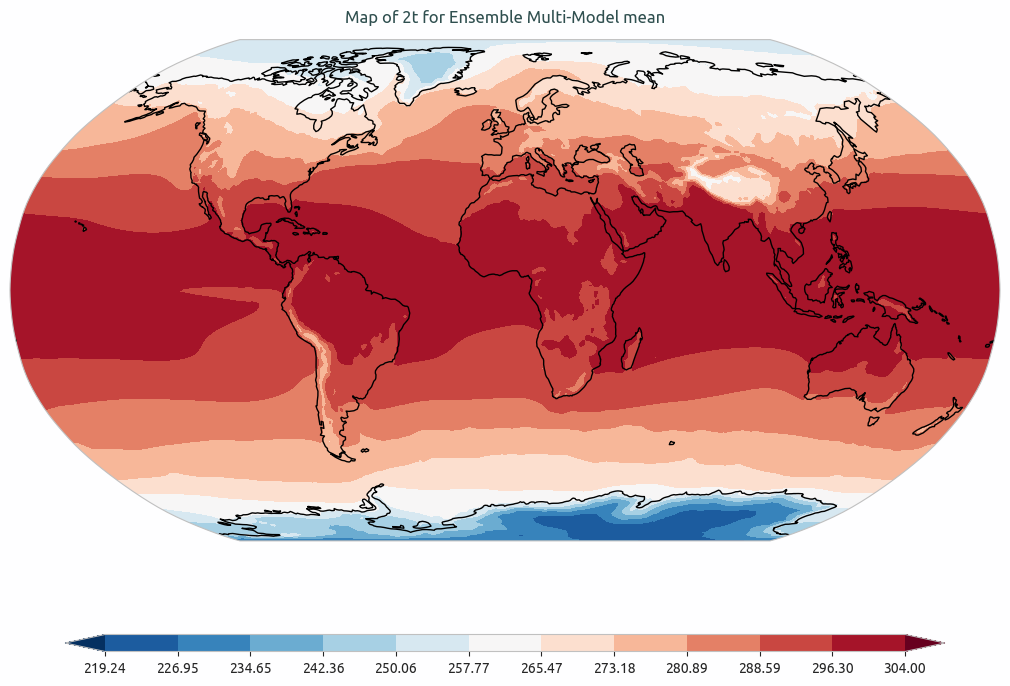
Ensemble mean of multi-model of global mean of 2-meter temperature. Models considered as IFS-NEMO and IFS-FESOM.
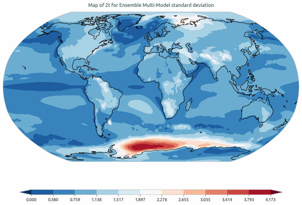
Ensemble standard devation of multi-model of the global mean of 2-meter temperature. Models considered as IFS-NEMO and IFS-FESOM.
Available demo notebooks
Notebooks are stored in the notebooks/diagnostics/ensemble directory and contain usage examples.
Detailed API
This section provides a detailed reference for the Application Programming Interface (API) of the Ensemble LatLon diagnostic,
produced from the diagnostic function docstrings.
Note
WORK IN PROGRESS