ECmean4 Performance Metrics

Description

ECmean4 is an open-source Python package integrated into AQUA to compute a set of baseline performance metrics for climate-model evaluation. It provides two complementary metrics:

the Reichler & Kim Performance Indices (PIs)
the Global Means (GMs)

Together, these metrics quantify the climatological skill of atmospheric and oceanic fields relative to observations.

Performance Indices (PIs)

PIs follow the Reichler and Kim (2008) Reichler and Kim Performance Indices, definition, with the adjustments implemented in ECmean4. For reference, see also * Reichler, T., and J. Kim, 2008: How Well Do Coupled Models Simulate Today’s Climate?. Bull. Amer. Meteor. Soc., 89, 303-312, https://doi.org/10.1175/BAMS-89-3-303. Key differences from the original formulation include:

metrics are computed on a common grid (1x1 deg) instead of the model grid
updated reference climatologies
PI estimates available for multiple regions and seasons

Formally, each PI is defined as the root-mean-square error (RMSE) of a 2D field normalized by the interannual variance of the corresponding observations. Higher values indicate poorer performance (i.e. larger bias). In ECmean4 plots, PIs are normalized by the precomputed average of CMIP6 climate models: values < 1 indicate a better performance than the CMIP6 average.

Global Means (GMs)

The GM metric consists of global averages of sany dynamical and physical fields, compared against a set of pre-computed climatological values for both the atmosphere and the ocean (e.g. land temperature, salinity, etc.). Multiple observational datasets are taken in consideration for each variable, providing an estimate of the plausible variability in the form of interannual standard deviation. GMs provides also estimate for the radiative budget and for the hydrological cycle (including integrals over land and ocean) and other quantities useful for fast model assessment and for model tuning.

Classes

For detailed information on the code, please refer to the official ECmean4 documentation.

File structure

The diagnostic is located in the aqua/diagnostics/ecmean directory, which contains the command line interface (CLI) script cli_ecmean.py.
A template configuration file is available at aqua/diagnostics/templates/diagnostics/config-ecmean.yaml
The configuration file for ECmean4 specific settings (variables and regions) is located in aqua/diagnostics/config/tools/ecmean/ecmean_config_climatedt.yaml.
The interface file to map AQUA variable names to ECmean4 standard names is located in aqua/diagnostics/config/tools/ecmean/interface/interface_AQUA_climatedt.yaml.
Notebooks are available in the notebooks/diagnostics/ecmean directory and contain examples of how to use the diagnostic.

For detailed information on the code, please refer to the official ECmean4 documentation.

Input variables and datasets

For Performance Indices the following variables are requested:

mtpr (Mean total precipitation rate, GRIB paramid 235055)
2t (2 metre temperature, GRIB paramid 167)
msl (mean sea level pressure, GRIB paramid 151)
metss (eastward wind stress, GRIB paramid 180)
mntss (northward wind stress, GRIB paramid 181)
t (air temperature, GRIB paramid 130)
u (zonal wind, GRIB paramid 131)
v (meridional wind, GRIB paramid 132)
q (specific humidity, GRIB paramid 133)
avg_tos (sea surface temperature, GRIB paramid 263101)
avg_sos (sea surface salinity, GRIB paramid 263100)
avg_siconc (sea ice concentration, GRIB paramid 263001)
msshf (surface sensible heat flux, GRIB paramid 235033, required for net surface flux computation)
mslhf` (surface latent heat flux, GRIB paramid 235034, required for net surface flux computation)
msnlwrf (surface net longwave radiation flux, GRIB paramid 235038, required for net surface flux computation)
msnswrf (surface net shortwave radiation flux, GRIB paramid 235037, required for net surface flux computation)
msr (snowfall rate, GRIB paramid 235031, required for net surface flux computation)

3D fields are zonally averaged, so that the PIs reports the performance on the zonal field.

For Global Means, the following variables are requested

mtpr (Mean total precipitation rate, GRIB paramid 235055)
mer (Mean evaporation rate, GRIB paramid 235043)
2t (2 metre temperature, GRIB paramid 167)
msl (mean sea level pressure, GRIB paramid 151)
metss (eastward wind stress, GRIB paramid 180)
mntss (northward wind stress, GRIB paramid 181)
t (air temperature, GRIB paramid 130)
u (zonal wind, GRIB paramid 131)
v (meridional wind, GRIB paramid 132)
q (specific humidity, GRIB paramid 133)
tcc (total cloud cover, GRIB paramid 228164)
mtnswrf (top net shortwave radiation, GRIB paramid 235039)
mtnlwrf (top net longwave radiation, GRIB paramid 235040)
avg_tos (sea surface temperature, GRIB paramid 263101)
avg_sos (sea surface salinity, GRIB paramid 263100)
avg_siconc (sea ice concentration, GRIB paramid 263001)
msshf (surface sensible heat flux, GRIB paramid 235033, required for net surface flux computation)
mslhf` (surface latent heat flux, GRIB paramid 235034, required for net surface flux computation)
msnlwrf (surface net longwave radiation flux, GRIB paramid 235038, required for net surface flux computation)
msnswrf (surface net shortwave radiation flux, GRIB paramid 235037, required for net surface flux computation)
msr (snowfall rate, GRIB paramid 235031, required for net surface flux computation)

For both diagnostics, if a variable (or more) is missing, blank line will be reported in the output figures.

Note

ECmean4 is made to work with CMOR variables, but can handle name and file conversion with specification of an interface file. An AQUA specific one has been designed for this purpose to work with Climate DT Phase 1. Updates in the Data Governance will require updates to the interface file. In addition, although PI and GM can work directly on the model raw output, the interface file is made to work only with the Low Resolution Archive (LRA) data, generated by the AQUA Data Reduction OPerator (DROP), to reduce the amount of computation required.

Basic usage

A complete example is provided in the notebooks/diagnostics/ecmean directory. The general structure of the analysis is the following:

import os
from aqua import Reader
from aqua.util import load_yaml, ConfigPath
from aqua.diagnostics import PerformanceIndices

models = ['IFS-NEMO', 'ICON']
exp = 'historical-1990'
year1 = 1996
year2 = 2000

Configurer = ConfigPath()
machine = Configurer.machine
ecmeandir = os.path.join(Configurer.configdir, 'diagnostics', 'ecmean')
interface = os.path.join(ecmeandir, 'interface_AQUA_climatedt.yaml')
config = os.path.join(ecmeandir, 'ecmean_config_climatedt.yaml')
config = load_yaml(config)

config['dirs']['exp'] = ecmeandir

for model in models:
    reader = Reader(model=model, exp=exp, source="lra-r100-monthly", fix=False)
    data = reader.retrieve()
    PerformanceIndices(exp, year1, year2, model=model, loglevel='info', xdataset=data, config=load_yaml(config))

Please refer also to the official ECmean4 documentation.

CLI usage

The diagnostic can be run from the command line interface (CLI) by running the following command:

cd $AQUA/aqua/diagnostics/ecmean
python cli_ecmean.py --config_file <path_to_config_file>

Additionally, the CLI can be run with the following optional arguments:

--config, -c: Path to the configuration file.
--nworkers, -n: Number of workers to use for parallel processing.
--cluster: Cluster to use for parallel processing. By default a local cluster is used.
--loglevel, -l: Logging level. Default is WARNING.
--catalog: Catalog to use for the analysis. Can be defined in the config file.
--model: Model to analyse. Can be defined in the config file.
--exp: Experiment to analyse. Can be defined in the config file.
--source: Source to analyse. Can be defined in the config file.
--outputdir: Output directory for the plots.
--nprocs: Number of multiprocessing processes to use.
--interface: Path to the interface file to use.
--source_ocean: Source of the oceanic data, to be used when oceanic data is in a different source than atmospheric data.

Configuration file structure

The configuration file is a YAML file that contains the details on the dataset to analyse or use as reference, the output directory and the diagnostic settings. Most of the settings are common to all the diagnostics (see Diagnostics configuration files). Here we describe only the specific settings for the ecmean diagnostic.

ecmean: a block (nested in the diagnostics block) containing options for the ECmean diagnostic. Variable-specific parameters override the defaults.
nprocs: number of multiprocessing processes to use (default: 1).
interface_file: path to the ECmean4 interface file to use.
config_file: path to the ECmean4 configuration file to use.

Two sub-blocks are available, one for Performance Indices and one for Global Means:

run: enable/disable the diagnostic.
diagnostic_name: name of the diagnostic. climate_metrics by default.
atm_vars: list of atmospheric variables to analyse for PIs and GMs.
oce_vars: list of oceanic variables to analyse for PIs and GMs.
year1 / year2: optional year range; if null, the full dataset is used.

diagnostics:
    ecmean:
        nprocs: 1
        interface_file: 'interface_AQUA_climatedt.yaml'
        config_file: 'ecmean_config_climatedt.yaml'

        global_mean:
        run: true
        diagnostic_name: 'climate_metrics'
        atm_vars: ['2t', 'tprate', 'msl', 'ie', 'iews', 'inss', 'tcc', 'tsrwe',
            'tnswrf', 'tnlwrf', 'snswrf', 'snlwrf', 'ishf', 'slhtf',
            'u', 'v', 't', 'q']
        oce_vars: ['tos', 'siconc', 'sos']
        year1: null #if you want to select some specific years, otherwise use the entire dataset
        year2: null

Output

The result are stored as a YAML file, indicating PIs and GMs for each variable, region and season, that can be stored for later evaluation. Most importantly, a figure for GMs and a figure for PIs (both in PDF format) are produced showing a score card for the different regions, variables and seasons. For the sake of simplicity, the PIs figure is computed as the ratio between the model PI and the average value estimated over the (precomputed) ensemble of CMIP6 models. Numbers lower than one imply that the model is performing better than the average of CMIP6 models.

Similarly, the GMs are reported as a score card with the average of the field, together with observational value reported in a smaller font, and colorscale which tells how many standard deviations from the interannual variability the model is far from observation. The whiter the color, the more reliable is the model output.

Reference datasets

ECmean4 uses multiple sources as reference climatologies: please refer to the climatology description for Performance Indices and for Global Mean to get more insight.

Example Plot(s)

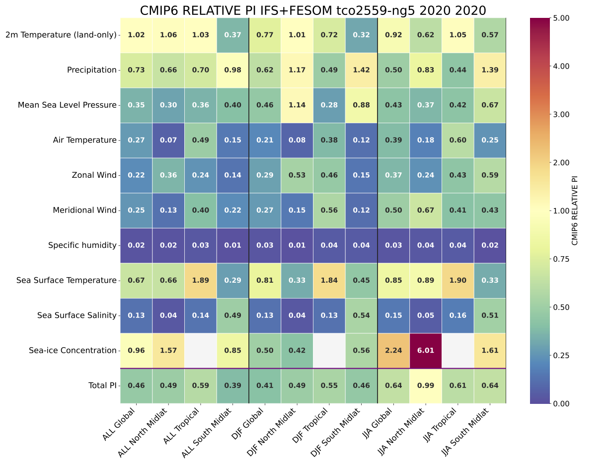
../_images/ecmean-pi.png — An example of the Performance Indices computed on a single year of the tco2599-ng5 simulation from NextGEMS Cycle2 run.

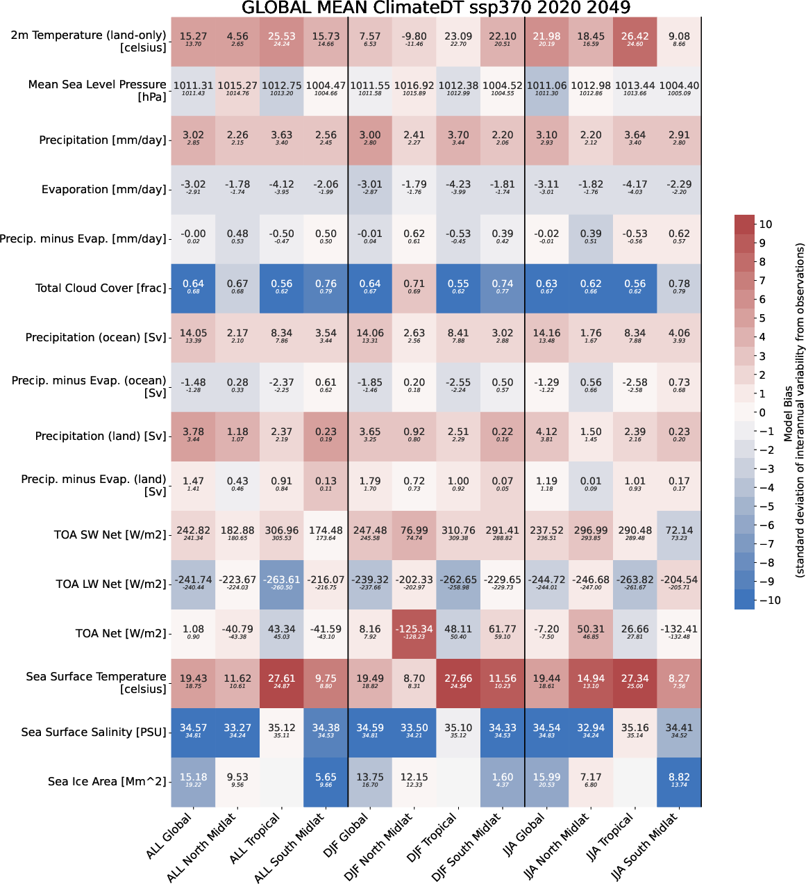
../_images/ecmean-gm.png — An example of the Global Mean computed on 30 years of the tco2599-ng5 simulation from NextGEMS Cycle4 run.

Available demo notebooks

Notebooks are stored in notebooks/diagnostics/ecmean.

ecmean-destine.ipynb

Authors and contributors

This diagnostic is maintained by Paolo Davini (@oloapinivad, paolo.davini@cnr.it). Contributions are welcome — please open an issue or a pull request. For questions or suggestions, contact the AQUA team or the maintainers.

Detailed API

This section provides a detailed reference for the Application Programming Interface (API) of the ecmean diagnostic, generated from the function docstrings.

class aqua.diagnostics.ecmean.GlobalMean(exp, year1, year2, config='config.yml', loglevel='WARNING', numproc=1, interface=None, model=None, ensemble='r1i1p1f1', addnan=False, silent=None, trend=None, line=None, outputdir=None, xdataset=None, reference='EC23', title=None)

Bases: object

exp

Experiment name.

Type:: str

year1

Start year of the experiment.

Type:: int

year2

End year of the experiment.

Type:: int

config

Path to the configuration file. Default is ‘config.yml’.

Type:: str

loglevel

Logging level. Default is ‘WARNING’.

Type:: str

numproc

Number of processes to use. Default is 1.

Type:: int

interface

Path to the interface file. Default is None.

Type:: str

model

Model name. Default is None.

Type:: str

ensemble

Ensemble identifier. Default is ‘r1i1p1f1’.

Type:: str

addnan

Whether to add NaNs. Default is False.

Type:: bool

silent

Whether to suppress output. Default is None.

Type:: bool

trend

Whether to compute trends. Default is None.

Type:: bool

line

Line identifier. Default is None.

Type:: str

outputdir

Output directory. Default is None.

Type:: str

xdataset

Path to the xdataset. Default is None.

Type:: str

loggy

Logger instance.

Type:: logging.Logger

diag

Diagnostic instance.

Type:: Diagnostic

face

Interface dictionary.

Type:: dict

ref

Reference dictionary.

Type:: dict

util_dictionary

Supporter instance.

Type:: Supporter

varmean

Dictionary to store variable means.

Type:: dict

vartrend

Dictionary to store variable trends.

Type:: dict

funcname

Name of the class.

Type:: str

start_time

Start time for the timer.

Type:: float

title

Title of the plot, overrides default title.

Type:: str

toc(message): Update the timer and log the elapsed time.

prepare(): Prepare the necessary components for the global mean computation.

run(): Run the global mean computation using multiprocessing.

store(): Store the computed global mean values in a table and YAML file.

plot(mapfile=None, figformat='pdf')

gm_worker(util, ref, face, diag, varmean, vartrend, varlist)

final_toc(): Log the total elapsed time since the start.

static gm_worker(util, ref, face, diag, varmean, vartrend, varlist, loglevel)

” Workhorse for the global mean computation.

Parameters:

util (Supporter) – Utility dictionary for remapping and masks.
ref (dict) – Reference climatology dictionary.
face (dict) – Interface dictionary.
diag (Diagnostic) – Diagnostic instance.
varmean (dict) – Shared dictionary to store variable means.
vartrend (dict) – Shared dictionary to store variable trends.
varlist (list) – List of variables to process.
varlist – List of variables to process.

plot(diagname='global_mean', mapfile=None, figformat='pdf', storefig=True, returnfig=False, addnan=True)

Generate the heatmap for global mean.

Parameters:

diagname (str) – Name of the diagnostic. Default is ‘global_mean’.
mapfile (str) – Path to the output file. If None, it will be defined automatically following ECmean syntax.
figformat (str) – Format of the output file. Default is ‘pdf’.
storefig (bool) – If True, store the figure in the specified file. Default is True.
returnfig (bool) – If True, return the figure object. Default is False.
addnan (bool) – If True, add NaN values to the plot. Default is True.

prepare(): Prepare the necessary components for the global mean computation.

run(): Run the global mean computaacross all variables on using multiprocessing.

store(yamlfile=None, tablefile=None): Rearrange the data and save the yaml file and the table. :param yamlfile: Path to the output YAML file. If None, it will be defined automatically. :param tablefile: Path to the output TXT file. If None, it will be defined automatically.

toc(message): Update the timer and log the elapsed time.

class aqua.diagnostics.ecmean.PerformanceIndices(exp, year1, year2, config='config.yml', loglevel='WARNING', numproc=1, climatology=None, interface=None, model=None, ensemble='r1i1p1f1', silent=None, xdataset=None, outputdir=None, extrafigure=False, title=None)

Bases: object

Class to compute the performance indices for a given experiment and years.

exp

Experiment name.

Type:: str

year1

Start year of the experiment.

Type:: int

year2

End year of the experiment.

Type:: int

config

Path to the configuration file. Default is ‘config.yml’.

Type:: str

loglevel

Logging level. Default is ‘WARNING’.

Type:: str

numproc

Number of processes to use. Default is 1.

Type:: int

climatology

Climatology to use. Default is ‘EC24’.

Type:: str

interface

Path to the interface file.

Type:: str

model

Model name.

Type:: str

ensemble

Ensemble identifier. Default is ‘r1i1p1f1’.

Type:: str

silent

If True, suppress output. Default is None.

Type:: bool

xdataset

Dataset to use.

Type:: xarray.Dataset

outputdir

Directory to store output files.

Type:: str

loggy

Logger instance.

Type:: logging.Logger

diag

Diagnostic instance.

Type:: Diagnostic

face

Interface dictionary.

Type:: dict

piclim

Climatology dictionary.

Type:: dict

util_dictionary

Utility dictionary for remapping and masks.

Type:: Supporter

varstat

Dictionary to store variable statistics.

Type:: dict

funcname

Name of the class.

Type:: str

start_time

Start time for performance measurement.

Type:: float

title

Title of the plot, overrides default title.

Type:: str

toc(message): Update the timer and log the elapsed time.

prepare(): Prepare the necessary components for performance indices calculation.

run(): Run the performance indices calculation.

store(yamlfile=None): Store the performance indices in a yaml file.

plot(mapfile=None, figformat='pdf'): Generate the heatmap for performance indices.

pi_worker(util, piclim, face, diag, field_3d, varstat, varlist): Main parallel diagnostic worker for performance indices.

Initialize the PerformanceIndices class with the given parameters.

final_toc(): Log the total elapsed time since the start.

static pi_worker(util, piclim, face, diag, field_3d, varstat, dictarray, varlist, loglevel)

Main parallel diagnostic worker for performance indices.

Parameters:

util (Supporter) – Utility dictionary for remapping and masks.
piclim (dict) – Climatology dictionary.
face (dict) – Interface dictionary.
diag (Diagnostic) – Diagnostic instance.
field_3d (list) – List of 3D fields.
varstat (dict) – Dictionary to store variable statistics.
dictarray (dict) – Dictionary to store the output array.
varlist (list) – List of variables to process.

plot(diagname='performance_indices', mapfile=None, figformat='pdf', storefig=True, returnfig=False)

Generate the heatmap for performance indices.

Parameters:

diagname (str) – Name of the diagnostic. Default is ‘performance_indices’.
mapfile (str) – Path to the output file. If None, it will be defined automatically following ECmean syntax.
storefig (bool) – If True, store the figure in the specified file. Default is True.
returnfig (bool) – If True, return the figure object. Default is False.

prepare(): Prepare the necessary components for performance indices calculation.

run(): Run the performance indices calculation.

store(yamlfile=None): Store the performance indices in a yaml file.

toc(message): Update the timer and log the elapsed time.