LatLonProfiles Diagnostic

Description

The LatLonProfiles diagnostic computes and plots zonally or meridionally averaged profiles of climate variables.

LatLonProfiles provides tools to plot:

• Zonal mean profiles (averaged over longitude, showing latitude profiles)

• Meridional mean profiles (averaged over latitude, showing longitude profiles)

• Seasonal profiles (4-panel: DJF, MAM, JJA, SON)

• Long-term mean profiles (single panel)

Profiles can be computed over specific geographic regions, with default regions available or custom regions definable in the configuration file.

The diagnostic is designed with a class that analyzes a single model and generates the NetCDF files, and another class that produces the plots.

Classes

There is one class for the analysis and one for the plotting:

• LatLonProfiles: retrieves the data and computes zonally or meridionally averaged profiles of climate variables. It handles spatial averaging, temporal averaging (seasonal or long-term), and optional standard deviation calculation for uncertainty analysis. Profiles are saved as class attributes and as NetCDF files.

• PlotLatLonProfiles: Produces publication-quality line plots of the computed profiles. It generates single-panel plots for long-term means and 4-panel plots for seasonal comparisons. It supports multiple model comparison with optional reference data and ±2σ uncertainty bands.

Note

The diagnostic follows a two-step process: spatial averaging (zonal/meridional) → temporal averaging (seasonal/long-term).

File structure

• The diagnostic is located in the aqua/diagnostics/lat_lon_profiles directory, which contains both the source code and the command line interface (CLI) script.

• A template configuration file is available at aqua/diagnostics/templates/diagnostics/config-lat_lon_profiles.yaml.

• Regional definitions are available in aqua/diagnostics/config/tools/lat_lon_profiles/definitions/regions.yaml.

• Notebooks are available in the notebooks/diagnostics/lat_lon_profiles directory and contain examples of how to use the diagnostic.

Input variables and datasets

The diagnostic works with climate variables on regular latitude-longitude grids.

Some of the variables that are typically used in this diagnostic are:

• 2t (2 metre temperature)

• tprate (total precipitation rate)

Derived variables can be computed using the EvaluateFormula syntax (e.g., 2t - 273.15 for temperature in °C).

Supported regions include: global (or null), tropics, europe, nh (Northern Hemisphere), sh (Southern Hemisphere). Custom regions can be defined in aqua/diagnostics/config/tools/lat_lon_profiles/definitions/regions.yaml.

The diagnostic is designed to work with data from the Low Resolution Archive (LRA), generated by the Data Reduction OPerator (DROP) of the AQUA project, which provides monthly data at a 1x1 degree resolution.

Basic usage

The basic usage of this diagnostic is explained with a working example in the notebook. The basic structure of the analysis is the following:

from aqua.diagnostics.lat_lon_profiles import LatLonProfiles, PlotLatLonProfiles

lonlat_dataset = LatLonProfiles(
    catalog='climatedt-phase1',
    model='ICON',
    exp='historical-1990',
    source='lra-r100-monthly',
    startdate='1990-01-01',
    enddate='1999-12-31'
    region='tropics',
    mean_type='zonal'  # or 'meridional'
)
lonlat_dataset.run(var='tprate', units='mm/day')

# Plot long-term mean
plot = PlotLatLonProfiles(data=[lonlat_dataset.longterm], data_type='longterm')
plot.run(show=True)

Note

Start/end dates and reference dataset can be customized. If not specified otherwise, plots will be saved in PNG and PDF format in the current working directory.

CLI usage

The diagnostic can be run from the command line interface (CLI) by running the following command:

cd $AQUA/aqua/diagnostics/lat_lon_profiles
python cli_lat_lon_profiles.py --config <path_to_config_file>

Additionally, the CLI can be run with the following optional arguments:

• --config, -c: Path to the configuration file.

• --nworkers, -n: Number of workers to use for parallel processing.

• --cluster: Cluster to use for parallel processing. By default a local cluster is used.

• --loglevel, -l: Logging level. Default is WARNING.

• --catalog: Catalog to use for the analysis. Can be defined in the config file.

• --model: Model to analyse. Can be defined in the config file.

• --exp: Experiment to analyse. Can be defined in the config file.

• --source: Source to analyse. Can be defined in the config file.

• --outputdir: Output directory for the plots.

• --startdate: Start date for the analysis.

• --enddate: End date for the analysis.

Configuration file structure

The configuration file is a YAML file that contains the details on the dataset to analyse or use as reference, the output directory and the diagnostic settings. Most of the settings are common to all the diagnostics (see Diagnostics configuration files). Here we describe only the specific settings for the lat_lon_profiles diagnostic.

• lat_lon_profiles: a block (nested in the diagnostics block) containing options for the LatLonProfiles diagnostic. Variable-specific parameters override the defaults.

  • run: enable/disable the diagnostic.

  • diagnostic_name: name of the diagnostic.

  • mean_type: type of spatial averaging (zonal or meridional).

  • seasonal: enable seasonal profiles computation.

  • longterm: enable long-term mean computation.

  • params: optional block of variable parameters. Contains a default sub-block with values applied to all variables, and optional per-variable sub-blocks (keyed by variable name) that override the defaults.

  • variables: list of variables to analyse with their regions. Inline values defined here take precedence over params.

diagnostics:
  lat_lon_profiles:
    run: true
    diagnostic_name: 'atmosphere2d'
    mean_type: 'zonal'
    center_time: true
    exclude_incomplete: true
    box_brd: true
    seasonal: true
    longterm: true
    params:
      default:
        std_startdate: '1990-01-01'
        std_enddate: '2019-12-31'
      2t:
        units: 'degC'
    variables:
      - name: '2t'
        regions: [null, 'tropics']  # global and tropics

Output

The diagnostic produces two types of plots:

• Long-term profiles (single panel)

• Seasonal profiles (4-panel: DJF, MAM, JJA, SON)

Plots are saved in both PDF and PNG format. Data outputs are saved as NetCDF files.

Observations

The default reference datasets are:

• ERA5 reanalysis for atmospheric variables

• MSWEP for precipitation data

• BERKELEY-EARTH for surface temperature

Details are available on the MSWEP website.

Standard deviation can be computed over a custom period using std_startdate and std_enddate to provide ±2σ uncertainty bands in plots. These dates can be set at three levels, in order of increasing priority: in the params.default block, in a per-variable params.<variable> block, or directly in the configuration of an individual dataset or reference.

Custom reference datasets can be configured in the configuration file.

Example plots

All plots can be reproduced using the notebooks in the notebooks directory on LUMI HPC.

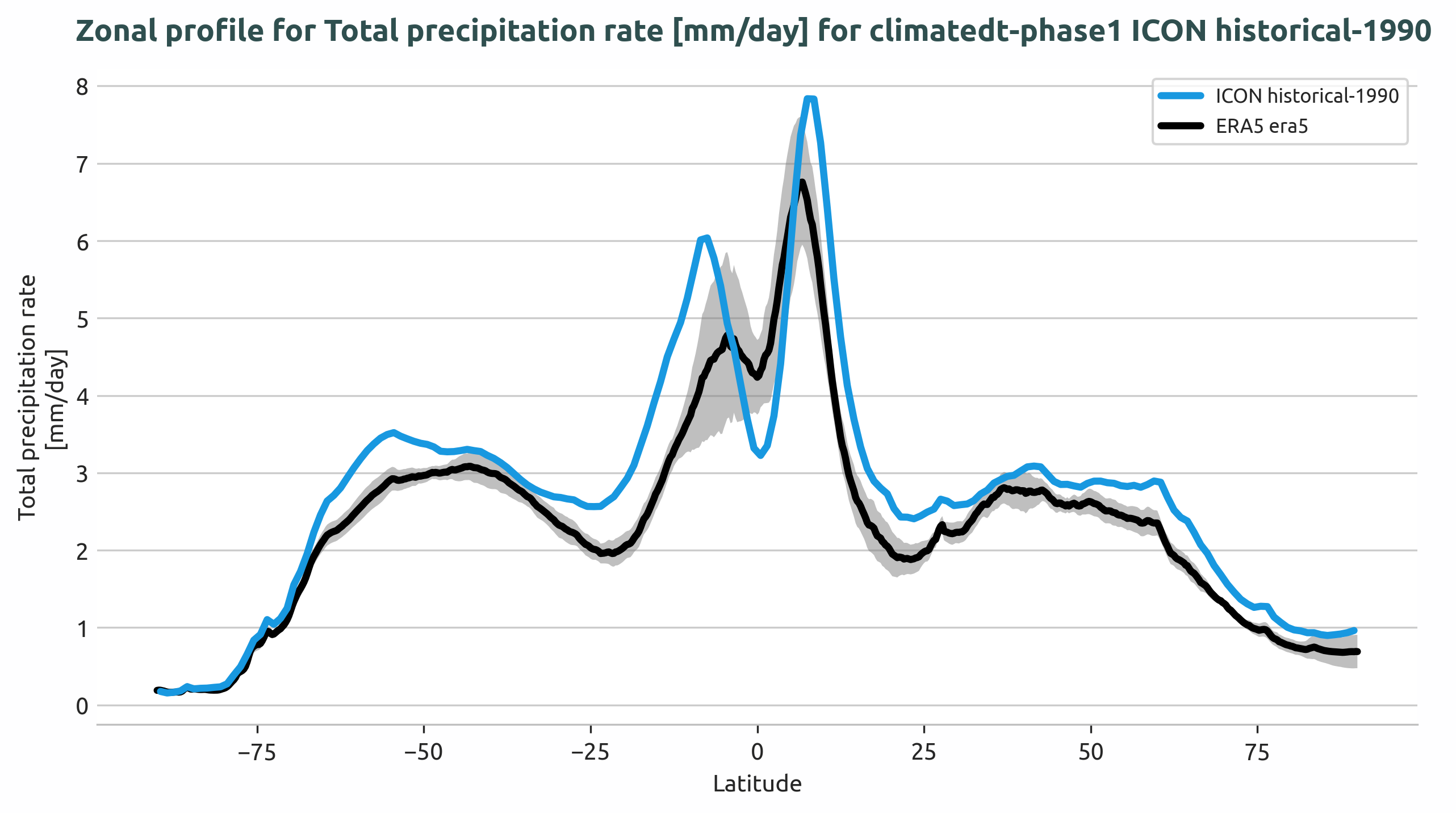
Long-term zonal mean precipitation rate profile for the Tropics region, showing ICON model output compared to ERA5 reference data with ±2σ uncertainty bands.

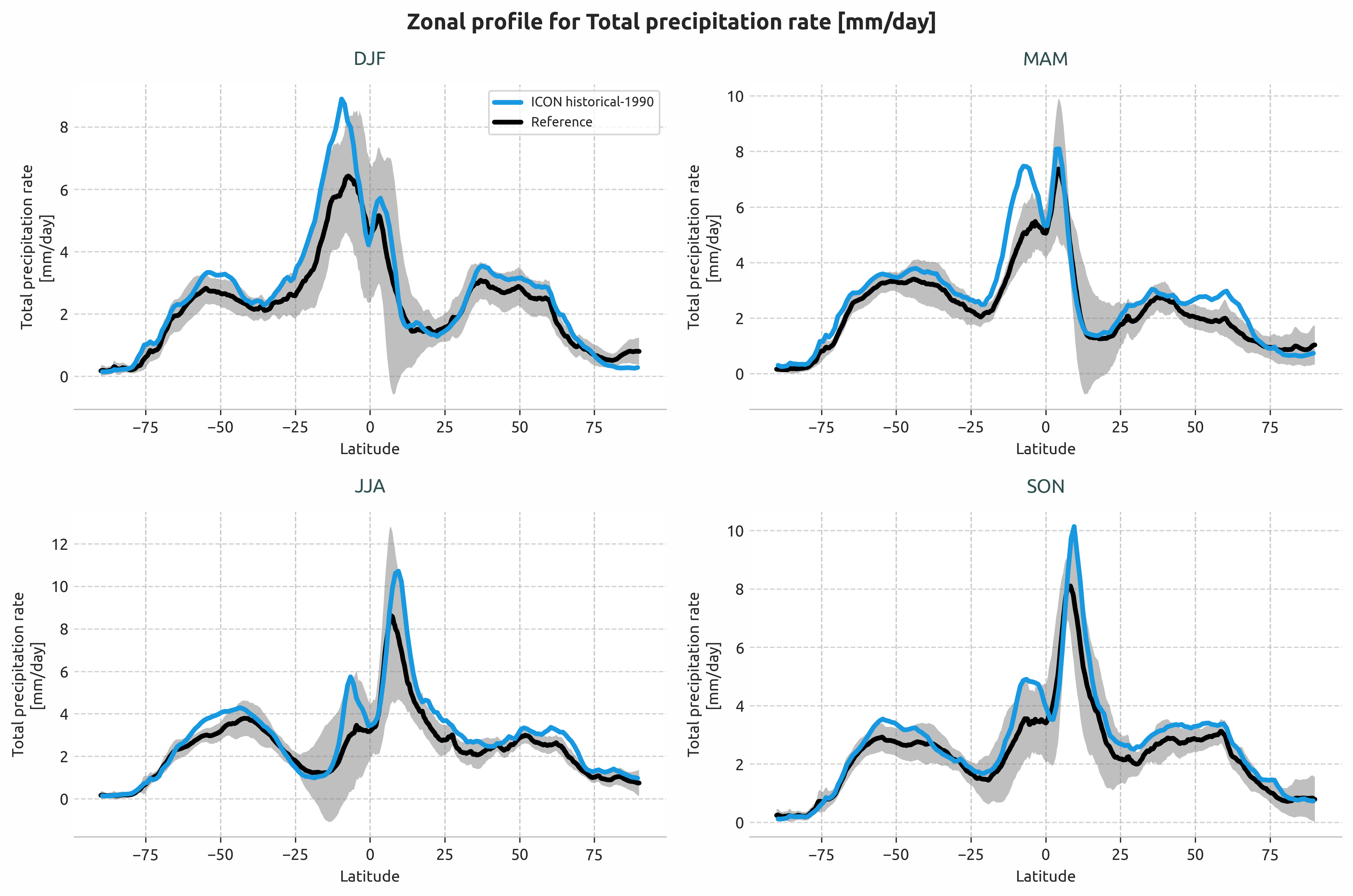
Seasonal zonal mean precipitation rate profiles (DJF, MAM, JJA, SON) for the Tropics region.

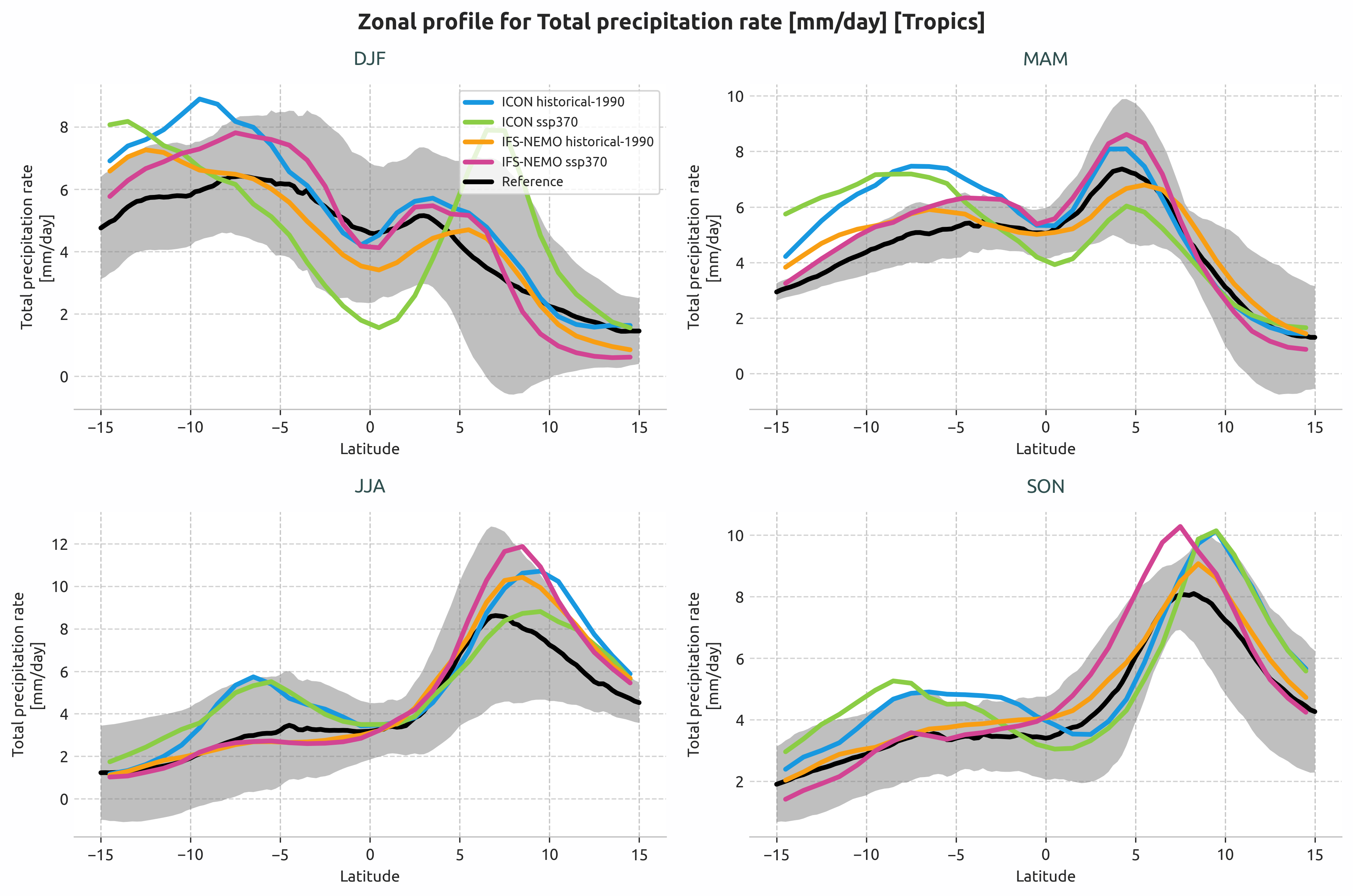
Multi-model comparison: ICON and IFS-NEMO historical and SSP3-7.0 scenarios.

Available demo notebooks

Notebooks are stored in notebooks/diagnostics/lat_lon_profiles:

• single_line_profiles.ipynb

• multiple_lines_profiles.ipynb

Authors and contributors

This diagnostic is maintained by Marco Cadau (@mcadau, marco.cadau@polito.it). Contributions are welcome — please open an issue or a pull request. For questions or suggestions, contact the AQUA team or the maintainers.

Detailed API

This section provides a detailed reference for the Application Programming Interface (API) of the lat_lon_profiles diagnostic, generated from the diagnostic function docstrings.

class aqua.diagnostics.lat_lon_profiles.LatLonProfiles(model: str, exp: str, source: str, catalog: str = None, regrid: str = None, startdate: str = None, enddate: str = None, std_startdate: str = None, std_enddate: str = None, region: str = None, lon_limits: list = None, lat_limits: list = None, regions_file_path: str = None, mean_type: str = 'zonal', diagnostic_name: str = 'latlonprofile', loglevel: str = 'WARNING')

Bases: Diagnostic

Class to compute lat-lon profiles of a variable over a specified region. It retrieves the data from the catalog, computes the mean and standard deviation over the specified period and saves the results to netcdf files.

Supported Frequencies:

• ‘seasonal’: Computes seasonal means (DJF, MAM, JJA, SON)

• ‘longterm’: Computes the temporal mean over the entire analysis period

Supported Mean Types:

• ‘zonal’: Average over longitude, producing latitude profiles

• ‘meridional’: Average over latitude, producing longitude profiles

Initialize the LatLonProfiles class.

Parameters:

• model (str) – The model to be used for the retrieval of the data.

• exp (str) – The experiment to be used for the retrieval of the data.

• source (str) – The source to be used for the retrieval of the data.

• catalog (str, optional) – The catalog to be used for the retrieval of the data.

• regrid (str, optional) – The regridding method to be used for the retrieval of the data.

• startdate (str, optional) – The start date of the plot/analysis period.

• enddate (str, optional) – The end date of the plot/analysis period.

• std_startdate (str, optional) – The start date of the standard deviation period.

• std_enddate (str, optional) – The end date of the standard deviation period.

• region (str, optional) – The region to be used for the retrieval of the data.

• lon_limits (list, optional) – The longitude limits of the region.

• lat_limits (list, optional) – The latitude limits of the region.

• regions_file_path (str, optional) – The path to the regions file. Default is the AQUA config path.

• mean_type (str, optional) – The type of mean to compute (‘zonal’ or ‘meridional’).

• diagnostic_name (str, optional) – The name of the diagnostic.

• loglevel (str, optional) – The log level to be used for the logging.

MINIMUM_MONTHS_REQUIRED = 12

compute_dim_mean(freq: str, exclude_incomplete: bool = True, center_time: bool = True, box_brd: bool = True)

Compute the mean of the data. Support for seasonal and longterm means.

Parameters:

• freq (str) – The frequency to be used (‘seasonal’ or ‘longterm’).

• exclude_incomplete (bool) – If True, exclude incomplete periods.

• center_time (bool) – If True, the time will be centered.

• box_brd (bool,opt) – choose if coordinates are comprised or not in area selection. Default is True

compute_std(freq: str, exclude_incomplete: bool = True, center_time: bool = True, box_brd: bool = True)

Compute the standard deviation of the data over the std period. Supports seasonal and longterm frequencies.

Parameters:

• freq (str) – The frequency to be used (‘seasonal’ or ‘longterm’).

• exclude_incomplete (bool) – If True, exclude incomplete periods.

• center_time (bool) – If True, the time will be centered.

• box_brd (bool,opt) – choose if coordinates are comprised or not in area selection. Default is True

retrieve(var: str, formula: bool = False, long_name: str = None, units: str = None, standard_name: str = None, reader_kwargs: dict = {})

Retrieve the data for the specified variable and apply any formula if required.

Parameters:

• var (str) – The variable to be retrieved.

• formula (bool) – Whether to use a formula for the variable.

• long_name (str) – The long name of the variable.

• units (str) – The units of the variable.

• standard_name (str) – The standard name of the variable.

• reader_kwargs (dict) – Additional keyword arguments for the Reader. Default is an empty dictionary.

run(var: str, formula: bool = False, long_name: str = None, units: str = None, standard_name: str = None, std: bool = False, freq: list = ['seasonal', 'longterm'], exclude_incomplete: bool = True, center_time: bool = True, box_brd: bool = True, outputdir: str = './', rebuild: bool = True, reader_kwargs: dict = {})

Run all the steps necessary for the computation of the LatLonProfiles.

Parameters:

• var (str) – The variable to be retrieved and computed.

• formula (bool) – Whether to use a formula for the variable.

• long_name (str) – The long name of the variable.

• units (str) – The units of the variable.

• standard_name (str) – The standard name of the variable.

• std (bool) – Whether to compute the standard deviation.

• freq (list) – The frequencies to compute. Options: - ‘seasonal’: Seasonal means (DJF, MAM, JJA, SON) - ‘longterm’: Long-term mean over the entire analysis period

• exclude_incomplete (bool) – Whether to exclude incomplete time periods.

• center_time (bool) – Whether to center the time coordinate.

• box_brd (bool) – Whether to include the box boundaries.

• outputdir (str) – The output directory to save the results.

• rebuild (bool) – Whether to rebuild existing files.

• reader_kwargs (dict) – Additional keyword arguments for the Reader. Default is an empty dictionary.

save_netcdf(freq: str, outputdir: str = './', rebuild: bool = True)

Save the data to a netcdf file.

Parameters:

• freq (str) – The frequency of the data (‘seasonal’ or ‘longterm’).

• outputdir (str) – The directory to save the data.

• rebuild (bool) – If True, rebuild the data from the original files.

class aqua.diagnostics.lat_lon_profiles.PlotLatLonProfiles(data=None, ref_data=None, data_type='longterm', ref_std_data=None, diagnostic_name='lat_lon_profiles', loglevel: str = 'WARNING')

Bases: object

Class for plotting Lat-Lon Profiles diagnostics. This class provides methods to set data labels, description, title, and to plot the data. It handles data arrays regardless of their original temporal frequency, as temporal averaging is handled upstream.

Initialise the PlotLatLonProfiles class. This class is used to plot lat lon profiles data previously processed by the LatLonProfiles class.

Parameters:

• data – Can be either: - List of temporally-averaged data arrays for annual plots - List of seasonal data [DJF, MAM, JJA, SON] for seasonal plots

• ref_data – Reference data (structure matches data based on data_type)

• data_type (str) – ‘longterm’ for single/multi-line longterm plots, ‘seasonal’ for 4-panel seasonal plots

• ref_std_data – Reference standard deviation data

• diagnostic_name (str) – Name of the diagnostic. Default is ‘lat_lon_profiles’.

• loglevel (str) – Logging level. Default is ‘WARNING’.

Note

data_type determines how ‘data’ is interpreted: - ‘longterm’: data should be list of DataArrays for single plot - ‘seasonal’: data should be [DJF, MAM, JJA, SON] for 4-panel seasonal plots

get_data_info()

Extract metadata from data arrays based on data_type.

plot(data_labels=None, ref_label=None, title=None, style=None)

Unified plotting method that handles all plotting scenarios based on data_type.

Parameters:

• data_labels (list, optional) – Labels for the data.

• ref_label (str, optional) – Label for the reference data.

• title (str, optional) – Title for the plot.

• style (str, optional) – Plotting style. Default is the AQUA style.

Returns:

Matplotlib figure and axes objects.

Return type:

tuple

plot_seasonal_lines(data_labels=None, title=None, style=None)

Plot seasonal means using plot_seasonal_lat_lon_profiles. Creates a 4-panel plot with DJF, MAM, JJA, SON only.

Parameters:

• data_labels (list) – List of data labels.

• title (str) – Title of the plot.

• style (str) – Plotting style. Default is the AQUA style

Returns:

Figure object. axs (list): List of axes objects.

Return type:

fig (matplotlib.figure.Figure)

run(outputdir='./', rebuild=True, dpi=300, style=None, format=['png', 'pdf', 'svg'], show=False)

Unified run method that handles all plotting scenarios.

Parameters:

• outputdir (str) – Output directory to save the plot.

• rebuild (bool) – If True, rebuild the plot even if it already exists.

• dpi (int) – Dots per inch for the plot.

• style (str) – Plotting style. Default is the AQUA style.

• format (str) – Format of the plot. Default is SAVE_FORMAT.

• show (bool) – If True, display the plot interactively.

save_plot(fig, description: str = None, rebuild: bool = True, outputdir: str = './', dpi: int = 300, format: str | list = ['png', 'pdf', 'svg'], diagnostic: str = None)

Save the plot to a file.

Parameters:

• fig (matplotlib.figure.Figure) – Figure object.

• description (str) – Description of the plot.

• rebuild (bool) – If True, rebuild the plot even if it already exists.

• outputdir (str) – Output directory to save the plot.

• dpi (int) – Dots per inch for the plot.

• format (str or list) – Format(s) to save the figure. Default is SAVE_FORMAT.

• diagnostic (str) – Diagnostic name to be used in the filename as diagnostic_product.

set_data_labels()

Set the data labels for the plot based on data_type.

set_description()

Set the caption for the plot.

set_ref_label()

Set the reference label for the plot. The label is extracted from the reference data array attributes.

Returns:

Reference label for the plot.

Return type:

ref_label (str)

set_title()

Set the title for the plot. Specialized for Lat-Lon Profiles diagnostic.

Returns:

Title for the plot.

Return type:

title (str)