Timeseries Diagnostic

Description

The Timeseries diagnostic is a set of tools to compute and plot time series, seasonal cycles and Gregory-like plot of a given variable or formula for a given model or list of models. Time series and seasonal cycles can be computed globally or for a specific area. The three functionalities are designed to have a class which analyse a single model to produce the netCDF files and another class to produce the plots. The diagnostic can compare the model time series with a reference dataset, which is defined in the configuration file.

Classes

There are three classes for the analysis:

Timeseries: computes time series of a given variable or formula for a given model or dataset. Comparison with a reference dataset is also possible. It supports hourly, daily, monthly and yearly time series and area selection. It can also compute the standard deviation of the time series.
SeasonalCycles: computes the seasonal cycle of a given variable or formula for a given model or dataset. Comparison with a reference dataset is also possible. It can also compute the standard deviation of the seasonal cycle. It supports area selection.
Gregory: computes the monthly and annual time series necessary for the Gregory-like plot of net radiation TOA and 2 metre temperature. It can also compute the standard deviation of the time series.

There are three other classes for the plotting:

PlotTimeseries: ingests xarrays and produces the plots for the time series. Info necessary for titles, legends and captions are deduced from the xarray attributes.
PlotSeasonalCycles: ingests xarrays and produces the plots for the seasonal cycle. Info necessary for titles, legends and captions are deduced from the xarray attributes.
PlotGregory: ingests xarrays and produces the Gregory-like plot. Info necessary for titles, legends and captions are deduced from the xarray attributes.

Warning

Hourly and daily plots are not available yet, while the netCDF files are produced.

File structure

The diagnostic is located in the aqua/diagnostics/timeseries directory, which contains both the source code and the command line interface (CLI) script.
A template configuration file is available at aqua/diagnostics/templates/diagnostics/config-timeseries.yaml
Notebooks are available in the notebooks/diagnostics/timeseries directory and contain examples of how to use the diagnostic.
A list of available regions is available in the aqua/diagnostics/config/tools/timeseries/definitions/regions.yaml file.

Input variables and datasets

By default, the diagnostic compares against the ERA5 dataset, with standard deviation calculated over the period 1990-2020. The Gregory-like plot uses the CERES dataset for the Net radiation TOA and the BERKELEY-EARTH dataset for the 2 metre temperature.

Default variables used for the timeseries and seasonal cycles analyses can be found in the configuration file. The Gregory-like plot requires the Net radiation TOA and the 2 metre temperature.

Basic usage

The basic usage of this diagnostic is explained with a working example in the notebook. The basic structure of the analysis is the following:

from aqua.diagnostics import Timeseries, PlotTimeseries

ts_dataset = Timeseries(catalog='climatedt-phase1',
            model= 'ICON',
            exp='historical-1990',
            source= 'lra-r100-monthly')

ts_obs = Timeseries(catalog='obs',
            model= 'ERA5',
            exp= 'era5',
            source= 'monthly',)

ts_dataset.run(var= '2t', units= 'degC')
ts_obs.run(var= '2t', units= 'degC', std=True)

plot_dict = {'monthly_data': ts_dataset.monthly,
              'annual_data': ts_dataset.annual,
              'ref_monthly_data': ts_obs.monthly,
              'ref_annual_data': ts_obs.annual,
              'std_monthly_data': ts_obs.std_monthly,
              'std_annual_data': ts_obs.std_annual,
              'loglevel': 'INFO'}

plot = PlotTimeseries(**plot_dict)
fig, _ = plot.plot_timeseries()

CLI usage

The diagnostic can be run from the command line interface (CLI) by running the following command:

cd $AQUA/aqua/diagnostics/timeseries
python cli_timeseries.py --config <path_to_config_file>

Three configuration files are provided and run when executing the aqua-analysis (see AQUA analysis wrapper).

Additionally CLI arguments are described in the Diagnostics CLI arguments section.

Configuration file structure

The configuration file is a YAML file that contains the details on the dataset to analyse or use as reference, the output directory and the diagnostic settings. Most of the settings are common to all the diagnostics (see Diagnostics configuration files). Here we describe only the specific settings for the time series diagnostic.

timeseries: a block, nested in the diagnostics block, that contains the details required for the time series. The parameters specific to a single variable are merged with the default parameters, giving priority to the specific ones.

diagnostics:
  timeseries:
    run: true # to enable the time series
    diagnostic_name: 'atmosphere'
    variables: ['2t', 'tprate']
    formulae: ['tnlwrf+tnswrf']
    center_time: true # center the time axis of the time series
    exclude_incomplete: true # check if all chunks are complete present before computing the time average
    params:
      default:
        hourly: false # Frequency to enable
        daily: false
        monthly: true
        annual: true
        std_startdate: '1990-01-01'
        std_enddate: '2020-12-31'
      tnlwrf+tnswrf:
        short_name: "net_top_radiation"
        long_name: "Net top radiation"
      tprate:
        units: 'mm/day'
        short_name: 'tprate'
        long_name: 'Total precipitation rate'
        regions: ['tropics', 'europe'] # regions to plot the time series other than global

seasonalcycles: a block, nested in the diagnostics block, that contains the details required for the seasonal cycle. The parameters specific to a single variable are merged with the default parameters, giving priority to the specific ones.

diagnostics:
  seasonalcycles:
    run: true # to enable the seasonal cycle
    diagnostic_name: 'atmosphere'
    variables: ['2t', 'tprate']
    center_time: true # center the time axis of the seasonal cycle
    exclude_incomplete: true # check if all chunks are complete present before computing the time average
    params:
      default:
        std_startdate: '1990-01-01'
        std_enddate: '2020-12-31'
      tprate:
        units: 'mm/day'
        long_name: 'Total precipitation rate'

gregory: a block, nested in the diagnostics block, that contains the details required for the Gregory-like plot.

diagnostics:
  gregory:
    run: true # to enable the Gregory plot
    diagnostic_name: 'climate_metrics'
    t2m: '2t' # variable name for the 2 metre temperature
    net_toa_name: 'tnlwrf+tnswrf' # formula or variable name for the Net radiation TOA
    monthly: true
    annual: true
    std: true
    std_startdate: '1990-01-01'
    std_enddate: '2020-12-31'
    # Gregory needs 2 datasets and do not care about the references block above
    t2m_ref: {'catalog': 'obs', 'model': 'BERKELEY-EARTH', 'exp': 'aqua-filled', 'source': 'r100-monthly'}
    net_toa_ref: {'catalog': 'obs', 'model': 'CERES', 'exp': 'ebaf-toa421', 'source': 'monthly'}

Output

The diagnostic produces three types of plots (see Example Plots):

A comparison of monthly and/or annual global mean time series of the model and the reference dataset.
A comparison of the seasonal cycle of the model and the reference dataset.
A Gregory-like plot of the model and the reference dataset as bands.

The timeseries, reference timeseries and standard deviation timeseries are also saved in the output directory as netCDF files.

Observations

The default reference dataset is ERA5 reanalysis, provided by ECMWF.

The diagnostic uses ERA5 monthly averages from the AQUA obs catalog (model=ERA5, exp=era5, source=monthly) for the global mean time series and seasonal cycle.

The Gregory-like plot uses BERKELEY-EARTH for the 2m temperature and CERES for the Net radiation TOA.

Custom reference datasets can be configured in the configuration file.

Note

Multiple reference time series and seasonal cycles plot are planned for the future.

Example Plots

A plot for each class is shown below. All these plots can be produced by running the notebooks in the notebooks directory on LUMI HPC.

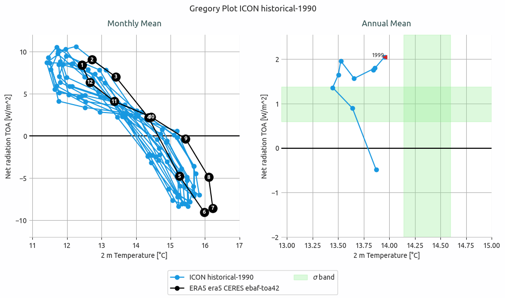
../_images/gregory_doc.png — Gregory plot of ICON historical-1990 simulation.

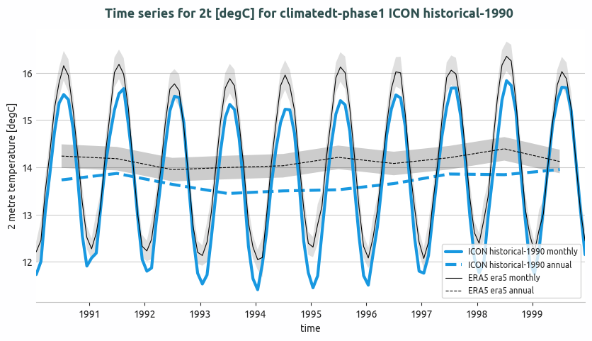
../_images/timeseries_doc.png — Global mean temperature time series of ICON historical-1990 and comparison with ERA5. Both monthly and annual timeseries are shown. A 2 sigma confidence interval is evaluated for ERA5 data (1990-2020).

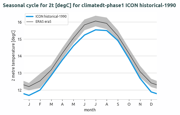
../_images/seasonalcycles_doc.png — Seasonal cycle of the global mean temperature of IFS-NEMO historical-1990 and comparison with ERA5. The 2 sigma confidence interval is evaluated for ERA5 data (1990-2020).

Available demo notebooks

Notebooks are stored in notebooks/diagnostics/timeseries:

Authors and contributors

This diagnostic is maintained by Matteo Nurisso (@mnurisso, matteo.nurisso@polito.it). Contributions are welcome — please open an issue or a pull request. For questions or suggestions, contact the AQUA team or the maintainer.

Detailed API

This section provides a detailed reference for the Application Programming Interface (API) of the timeseries diagnostic, produced from the diagnostic function docstrings.

class aqua.diagnostics.timeseries.Gregory(diagnostic_name: str = 'gregory', catalog: str = None, model: str = None, exp: str = None, source: str = None, regrid: str = None, startdate: str = None, enddate: str = None, loglevel: str = 'WARNING')

Bases: Diagnostic

Initialize the Gregory Plot class. This evaluates values necessary for the Gregory Plot from a single model and to save the data to a netcdf file.

Parameters:

catalog (str) – The catalog to be used. If None, the catalog will be determined by the Reader.
model (str) – The model to be used.
exp (str) – The experiment to be used.
source (str) – The source to be used.
regrid (str) – The target grid to be used for regridding. If None, no regridding will be done.
startdate (str) – The start date of the data to be retrieved. If None, all available data will be retrieved.
enddate (str) – The end date of the data to be retrieved. If None, all available data will be retrieved.
loglevel (str) – The log level to be used. Default is ‘WARNING’.

Initialize the diagnostic class. This is a general purpose class that can be used by the diagnostic classes to retrieve data from a single model and to save the data to a netcdf file. It is not a working diagnostic class by itself.

Parameters:

model (str) – The model to be used.
exp (str) – The experiment to be used.
source (str) – The source to be used.
catalog (str) – The catalog to be used. If None, the catalog will be determined by the Reader.
regrid (str | None) – The target grid to be used for regridding. If None, no regridding will be done.
startdate (str | None) – The start date of the plot/analysis period. If None, all available data will be used.
enddate (str | None) – The end date of the plot/analysis period. If None, all available data will be used.
std_startdate (str | None) – The start date of the standard deviation period. If None, no std period is tracked at the Diagnostic level.
std_enddate (str | None) – The end date of the standard deviation period. If None, no std period is tracked at the Diagnostic level.
loglevel (str) – The log level to be used. Default is ‘WARNING’.

MINIMUM_MONTHS_REQUIRED = 2

compute_net_toa(freq: list = ['monthly', 'annual'], std: bool = False, exclude_incomplete=True)

Compute the net TOA radiation data.

Parameters:

freq (list) – The frequency of the data to be computed. Default is [‘monthly’, ‘annual’].
std (bool) – Whether to compute the standard deviation. Default is False.
exclude_incomplete (bool) – Whether to exclude incomplete timespans. Default is True.

compute_t2m(freq: list = ['monthly', 'annual'], std: bool = False, var: str = '2t', units: str = 'degC', exclude_incomplete=True)

Compute the 2m temperature data.

Parameters:

freq (list) – The frequency of the data to be computed. Default is [‘monthly’, ‘annual’].
std (bool) – Whether to compute the standard deviation. Default is False.
units (str) – The units of the data. Default is ‘degC’.
exclude_incomplete (bool) – Whether to exclude incomplete timespans. Default is True.

retrieve(t2m: bool = True, net_toa: bool = True, t2m_name: str = '2t', net_toa_name: str = 'tnlwrf+tnswrf', reader_kwargs: dict = {})

Retrieve the necessary data for the Gregory Plot.

Parameters:

t2m (bool) – Whether to retrieve the 2m temperature data. Default is True.
net_toa (bool) – Whether to retrieve the net TOA radiation data. Default is True.
t2m_name (str) – The name of the 2m temperature data.
net_toa_name (str) – The name of the net TOA radiation data.
reader_kwargs (dict) – Additional keyword arguments for the Reader. Default is an empty dictionary.

run(freq: list = ['monthly', 'annual'], t2m: bool = True, net_toa: bool = True, std: bool = False, t2m_name: str = '2t', net_toa_name: str = 'tnlwrf+tnswrf', t2m_units: str = 'degC', exclude_incomplete: bool = True, outputdir: str = './', rebuild: bool = True, reader_kwargs: dict = {})

Run the Gregory Plot.

Args:
freq (list): The frequency of the data to be computed. Default is [‘monthly’, ‘annual’]. t2m (bool): Whether to compute the 2m temperature data. Default is True. net_toa (bool): Whether to compute the net TOA radiation data. Default is True. std (bool): Whether to compute the standard deviation. Default is False. t2m_name (str): The name of the 2m temperature variable. Default is ‘2t’. net_toa_name (str): The name of the net TOA radiation formula. Default is ‘tnlwrf+tnswrf’. t2m_units (str): The units of the 2m temperature data. Default is ‘degC’. exclude_incomplete (bool): Whether to exclude incomplete timespans. Default is True. outputdir (str): The output directory to save the netcdf file. Default is ‘./’. rebuild (bool): Whether to rebuild the netcdf file. Default is True. reader_kwargs (dict): Additional keyword arguments for the Reader. Default is an empty dictionary.

save_netcdf(freq: list = ['monthly', 'annual'], std: bool = False, t2m: bool = True, net_toa: bool = True, outputdir: str = './', rebuild: bool = True)

Save the computed data to a netcdf file.

Parameters:

freq (list) – The frequency of the data to be saved. Default is [‘monthly’, ‘annual’].
std (bool) – Whether to save the standard deviation. Default is False.
t2m (bool) – Whether to save the 2m temperature data. Default is True.
net_toa (bool) – Whether to save the net TOA radiation data. Default is True.
outputdir (str) – The output directory to save the netcdf file. Default is ‘./’.
rebuild (bool) – Whether to rebuild the netcdf file. Default is True.

class aqua.diagnostics.timeseries.PlotGregory(diagnostic_name: str = 'gregory', t2m_monthly_data=None, net_toa_monthly_data=None, t2m_annual_data=None, net_toa_annual_data=None, t2m_monthly_ref=None, net_toa_monthly_ref=None, t2m_annual_ref=None, net_toa_annual_ref=None, t2m_annual_std=None, net_toa_annual_std=None, loglevel: str = 'WARNING')

Bases: PlotBaseMixin

Initialize the class with the data to be plotted

Parameters:

t2m_monthly_data – List of monthly 2m temperature data
net_toa_monthly_data – List of monthly net toa data
t2m_annual_data – List of annual 2m temperature data
net_toa_annual_data – List of annual net toa data
t2m_monthy_ref – Monthly reference 2m temperature data
net_toa_monthy_ref – Monthly reference net toa data
t2m_annual_ref – Aannual reference 2m temperature data
net_toa_annual_ref – Annual reference net toa data
t2m_annual_std – Annual standard deviation of 2m temperature data
net_toa_annual_std – Annual standard deviation of net toa data
loglevel – Logging level. Default is ‘WARNING’

get_data_info()

We extract the data needed for labels, description etc from the data arrays attributes.

The attributes are: - AQUA_catalog - AQUA_model - AQUA_exp

plot(freq=['monthly', 'annual'], title: str = None, data_labels: list = None, ref_label: str = None, style: str = 'aqua')

Plot the data

Parameters:

freq – List of frequency for plotting. Default is [‘monthly’, ‘annual’]
title – Title of the plot. Default is None
data_labels – List of labels for the data. Default is None
ref_label – Label for the reference data. Default is None
style – Style of the plot. Default is ‘aqua’

plot_annual(fig: Figure, ax: Axes, data_labels: list = None)

Plot the annual data

Parameters:

fig – Figure object
ax – Axes object
data_labels – List of labels for the data. Default is None

Returns:

Figure object ax: Axes object

Return type:

fig

plot_monthly(fig: Figure, ax: Axes, data_labels: list = None, ref_label: str = None)

Plot the monthly data

Parameters:

fig – Figure object
ax – Axes object
data_labels – List of labels for the data. Default is None
ref_label – Label for the reference data. Default is None

Returns:

Figure object ax: Axes object

Return type:

fig

set_description(): Set the description for the plot

set_ref_label(): Set the reference label for the plot

set_title(): Set the title for the plot

class aqua.diagnostics.timeseries.PlotSeasonalCycles(diagnostic_name: str = 'seasonalcycles', monthly_data=None, ref_monthly_data=None, std_monthly_data=None, loglevel: str = 'WARNING')

Bases: PlotBaseMixin

Initialize the PlotSeasonalCycles class. This class is used to plot seasonal cycles data previously processed by the SeasonalCycles class.

Parameters:

diagnostic_name (str) – The name of the diagnostic. Used for logger and filenames. Default is ‘seasonalcycles’.
monthly_data (list) – List of monthly data arrays.
ref_monthly_data (xr.DataArray) – Reference monthly data array.
std_monthly_data (xr.DataArray) – Standard deviation monthly data array.
loglevel (str) – Logging level. Default is ‘WARNING’.

get_data_info()

We extract the data needed for labels, description etc from the data arrays attributes.

The attributes are: - AQUA_catalog - AQUA_model - AQUA_exp - AQUA_startdate - AQUA_enddate - AQUA_std_startdate - AQUA_std_enddate - AQUA_region - short_name - long_name - units

plot_seasonalcycles(data_labels=None, ref_label=None, title=None)

Plot the seasonal cycle using the plot_seasonalcycle function.

Parameters:

data_labels (list) – List of data labels.
ref_label (str) – Reference label.
title (str) – Title of the plot.

Returns:

Figure object. ax (matplotlib.axes.Axes): Axes object.

Return type:

fig (matplotlib.figure.Figure)

run(outputdir: str = './', rebuild: bool = True, dpi: int = 300, format: str | list = ['png', 'pdf', 'svg'])

Run the PlotTimeseries class.

Parameters:

outputdir (str) – Output directory to save the plot.
rebuild (bool) – If True, rebuild the plot even if it already exists.
dpi (int) – Dots per inch for the plot.
format (str or list) – Format(s) to save the figure. Default is SAVE_FORMAT.

save_plot(fig, description: str | None = None, rebuild: bool = True, outputdir: str = './', dpi: int = 300, format: str | list = ['png', 'pdf', 'svg'])

Save the plot to a file.

Parameters:

fig (matplotlib.figure.Figure) – Figure object.
description (str, optional) – Description of the plot.
rebuild (bool) – If True, rebuild the plot even if it already exists.
outputdir (str) – Output directory to save the plot.
dpi (int) – Dots per inch for the plot.
format (str or list) – Format(s) to save the figure. Default is SAVE_FORMAT.

set_description()

Set the caption for the plot. The caption is extracted from the data arrays attributes and the reference data arrays attributes. The caption is stored as ‘Description’ in the metadata dictionary.

Returns:: Caption for the plot.
Return type:: description (str)

set_title()

Set the title for the plot.

Returns:: Title for the plot.
Return type:: title (str)

class aqua.diagnostics.timeseries.PlotTimeseries(diagnostic_name: str = 'timeseries', hourly_data=None, daily_data=None, monthly_data=None, annual_data=None, ref_hourly_data=None, ref_daily_data=None, ref_monthly_data=None, ref_annual_data=None, std_hourly_data=None, std_daily_data=None, std_monthly_data=None, std_annual_data=None, loglevel: str = 'WARNING')

Bases: PlotBaseMixin

Class to plot time series data.

Initialize the PlotTimeseries class. This class is used to plot time series data previously processed by the Timeseries class.

Any subset of frequency can be provided, however the order and length of the list of data arrays must be the same for each frequency.

Note: Currently, only monthly and annual data are supported. Additionally, only one reference data array is supported for each frequency.

Parameters:

diagnostic_name (str) – The name of the diagnostic. Used for logger and filenames. Default is ‘timeseries’.
hourly_data (list) – List of hourly data arrays.
daily_data (list) – List of daily data arrays.
monthly_data (list) – List of monthly data arrays.
annual_data (list) – List of annual data arrays.
ref_hourly_data (xr.DataArray) – Reference hourly data array.
ref_daily_data (xr.DataArray) – Reference daily data array.
ref_monthly_data (xr.DataArray) – Reference monthly data array.
ref_annual_data (xr.DataArray) – Reference annual data array.
std_hourly_data (xr.DataArray) – Standard deviation hourly data array.
std_daily_data (xr.DataArray) – Standard deviation daily data array.
std_monthly_data (xr.DataArray) – Standard deviation monthly data array.
std_annual_data (xr.DataArray) – Standard deviation annual data array.
loglevel (str) – Logging level. Default is ‘WARNING’.

get_data_info()

We extract the data needed for labels, description etc from the data arrays attributes.

The attributes are: - AQUA_catalog - AQUA_model - AQUA_exp - AQUA_region - AQUA_startdate - AQUA_enddate - AQUA_std_startdate - AQUA_std_enddate - short_name - long_name - units

plot_timeseries(data_labels=None, ref_label=None, title=None)

Plot the time series data.

Parameters:

data_labels (list) – List of data labels.
ref_label (str) – Reference label.
title (str) – Title of the plot.

Returns:

Figure object. ax (matplotlib.axes.Axes): Axes object.

Return type:

fig (matplotlib.figure.Figure)

run(outputdir: str = './', rebuild: bool = True, dpi: int = 300, format: str = 'png')

Run the PlotTimeseries class.

Parameters:

outputdir (str) – Output directory to save the plot.
rebuild (bool) – If True, rebuild the plot even if it already exists.
dpi (int) – Dots per inch for the plot.
format (str) – Format of the plot (‘png’ or ‘pdf’). Default is ‘png’.

save_plot(fig, description: str = None, rebuild: bool = True, outputdir: str = './', dpi: int = 300, format: str = 'png')

Save the plot to a file.

Parameters:

fig (matplotlib.figure.Figure) – Figure object.
description (str) – Description of the plot.
rebuild (bool) – If True, rebuild the plot even if it already exists.
outputdir (str) – Output directory to save the plot.
dpi (int) – Dots per inch for the plot.
format (str) – Format of the plot (‘png’ or ‘pdf’). Default is ‘png’.

set_description()

Set the caption for the plot. The caption is extracted from the data arrays attributes and the reference data arrays attributes. The caption is stored as ‘Description’ in the metadata dictionary.

Returns:: Caption for the plot.
Return type:: description (str)

set_title()

Set the title for the plot.

Returns:: Title for the plot.
Return type:: title (str)

class aqua.diagnostics.timeseries.SeasonalCycles(diagnostic_name: str = 'seasonalcycles', catalog: str = None, model: str = None, exp: str = None, source: str = None, regrid: str = None, startdate: str = None, enddate: str = None, std_startdate: str = None, std_enddate: str = None, region: str = None, lon_limits: list = None, lat_limits: list = None, loglevel: str = 'WARNING')

Bases: BaseMixin

SeasonalCycles class for retrieve and netcdf saving of a single experiment

Initialize the Timeseries class.

Parameters:

diagnostic_name (str) – The name of the diagnostic. Used for logger and filenames. Default is ‘seasonalcycles’.
catalog (str) – The catalog to be used. If None, the catalog will be determined by the Reader.
model (str) – The model to be used.
exp (str) – The experiment to be used.
source (str) – The source to be used.
regrid (str) – The target grid to be used for regridding. If None, no regridding will be done.
startdate (str) – The start date of the data to be retrieved. If None, all available data will be retrieved.
enddate (str) – The end date of the data to be retrieved. If None, all available data will be retrieved.
std_startdate (str) – The start date of the standard deviation evaluation period.
std_enddate (str) – The end date of the standard deviation evaluation period.
region (str) – The region to select. This will define the lon and lat limits.
lon_limits (list) – The longitude limits to be used. Overriden by region.
lat_limits (list) – The latitude limits to be used. Overriden by region.
loglevel (str) – The log level to be used. Default is ‘WARNING’.

MINIMUM_MONTHS_REQUIRED = 2

compute(exclude_incomplete: bool = True, center_time: bool = True, box_brd: bool = True)

Compute the seasonal cycles.

Parameters:

exclude_incomplete (bool) – If True, exclude incomplete periods.
center_time (bool) – If True, the time will be centered.
box_brd (bool) – choose if coordinates are comprised or not in area selection.

run(var: str, formula: bool = False, long_name: str = None, units: str = None, short_name: str = None, std: bool = False, exclude_incomplete: bool = True, center_time: bool = True, box_brd: bool = True, outputdir: str = './', rebuild: bool = True, reader_kwargs: dict = {}, create_catalog_entry: bool = False)

Run all the steps necessary for the computation of the SeasonalCyles. Save the results to netcdf files.

Parameters:

var (str) – The variable to be used.
formula (bool) – If True, the variable is a formula.
long_name (str) – The long name of the variable, if different from the variable name.
units (str) – The units of the variable, if different from the original units.
short_name (str) – The short name of the variable, if different from the variable name.
std (bool) – If True, compute the standard deviation. Default is False.
exclude_incomplete (bool) – If True, exclude incomplete periods.
center_time (bool) – If True, the time will be centered.
box_brd (bool) – choose if coordinates are comprised or not in area selection.
outputdir (str) – The directory to save the data.
rebuild (bool) – If True, rebuild the data.
reader_kwargs (dict) – Additional keyword arguments for the Reader. Default is an empty dictionary.
create_catalog_entry (bool) – If True, create a catalog entry for the data. Default is False.

class aqua.diagnostics.timeseries.Timeseries(diagnostic_name: str = 'timeseries', catalog: str = None, model: str = None, exp: str = None, source: str = None, regrid: str = None, startdate: str = None, enddate: str = None, std_startdate: str = None, std_enddate: str = None, region: str = None, lon_limits: list = None, lat_limits: list = None, loglevel: str = 'WARNING')

Bases: BaseMixin

Timeseries class for retrieve and netcdf saving of a single experiment

Initialize the Timeseries class.

Parameters:

diagnostic_name (str) – The name of the diagnostic. Used for logger and filenames. Default is ‘timeseries’.
catalog (str) – The catalog to be used. If None, the catalog will be determined by the Reader.
model (str) – The model to be used.
exp (str) – The experiment to be used.
source (str) – The source to be used.
regrid (str) – The target grid to be used for regridding. If None, no regridding will be done.
startdate (str) – The start date of the data to be retrieved. If None, all available data will be retrieved.
enddate (str) – The end date of the data to be retrieved. If None, all available data will be retrieved.
std_startdate (str) – The start date of the standard period.
std_enddate (str) – The end date of the standard period.
region (str) – The region to select. This will define the lon and lat limits.
lon_limits (list) – The longitude limits to be used. Overriden by region.
lat_limits (list) – The latitude limits to be used. Overriden by region.
loglevel (str) – The log level to be used. Default is ‘WARNING’.

MINIMUM_MONTHS_REQUIRED = 2

compute(freq: str, exclude_incomplete: bool = True, center_time: bool = True, box_brd: bool = True)

Compute the mean of the data. Support for hourly, daily, monthly and annual means.

Parameters:

freq (str) – The frequency to be used for the resampling.
exclude_incomplete (bool) – If True, exclude incomplete periods.
center_time (bool) – If True, the time will be centered.
box_brd (bool,opt) – choose if coordinates are comprised or not in area selection. Default is True

run(var: str, formula: bool = False, long_name: str = None, units: str = None, short_name: str = None, std: bool = False, freq: list = ['monthly', 'annual'], exclude_incomplete: bool = True, center_time: bool = True, box_brd: bool = True, outputdir: str = './', rebuild: bool = True, reader_kwargs: dict = {}, create_catalog_entry: bool = False)

Run all the steps necessary for the computation of the Timeseries. Save the results to netcdf files. Can evaluate different frequencies.

Parameters:

var (str) – The variable to be retrieved.
formula (bool) – If True, the variable is a formula.
long_name (str) – The long name of the variable, if different from the variable name.
units (str) – The units of the variable, if different from the original units.
short_name (str) – The short name of the variable, if different from the variable name.
std (bool) – If True, compute the standard deviation. Default is False.
freq (list) – The frequencies to be used for the computation. Available options are ‘hourly’, ‘daily’, ‘monthly’ and ‘annual’. Default is [‘monthly’, ‘annual’].
exclude_incomplete (bool) – If True, exclude incomplete periods.
center_time (bool) – If True, the time will be centered.
box_brd (bool) – choose if coordinates are comprised or not in area selection.
outputdir (str) – The directory to save the data.
rebuild (bool) – If True, rebuild the data from the original files.
reader_kwargs (dict) – Additional keyword arguments for the Reader. Default is an empty dictionary.
create_catalog_entry (bool) – If True, create a catalog entry for the data. Default is False.