Ocean Trends Diagnostic

Description

The OceanTrends diagnostic is a set of tools for the analysis and visualization of linear trends in ocean model outputs over time. It computes temporal trends for ocean variables at different depths and provides spatial representations of these trends. The diagnostic is designed to identify systematic changes in ocean properties, which can indicate climate drift, model bias evolution, or physical climate change signals.

OceanTrends provides tools to:

Compute linear trends over time for ocean variables
Generate multi-level spatial maps showing trend patterns at different depths
Produce zonal mean vertical sections of trends, particularly useful for identifying depth-dependent trend structures

The diagnostic is designed with a class that computes trend coefficients from ocean data, and another class that produces the plots.

Classes

There are two main classes for analysis and plotting:

Trends: retrieves ocean data and computes linear trend coefficients over time using polynomial fitting. It handles temporal frequency detection, automatic unit conversion to trends per year, and spatial averaging or region selection. The diagnostic performs a polynomial fit of degree 1 (linear fit) to the time series at each grid point, after normalizing the time coordinate. Final trend units are expressed as [original_units]/year The Trender class from AQUA’s core library, which implements robust polynomial fitting with the option to skip NaN values. Results are saved as class attributes and as NetCDF files. Regions can be predefined (e.g., Atlantic Ocean, Pacific Ocean, Global Ocean) or custom-defined by the user.
PlotTrends: provides methods for plotting trend coefficients as spatial maps and zonal mean vertical sections. It generates multi-level plots showing trend patterns at different depths and multi-variable comparisons.

File structure

The diagnostic is located in the aqua/diagnostics/ocean_trends directory, which contains both the source code and the command line interface (CLI) script.
A template configuration file is available at aqua/diagnostics/templates/diagnostics/config-trends.yaml
Notebooks are available in the notebooks/diagnostics/trends directory and contain examples of how to use the diagnostic.

Input variables and datasets

The diagnostic works with 3D ocean model outputs and can be applied to any ocean variable.

The primary variables typically used in this diagnostic are:

thetao (sea water potential temperature)
so (sea water salinity)

The diagnostic is designed to work with data from the Low Resolution Archive (LRA), generated by the Data reduction OPerator (DROP) of the AQUA project, which provides monthly data at a 1x1 degree resolution. A higher resolution is not necessary for this diagnostic.

Basic usage

The basic usage of this diagnostic is explained with a working example in the notebook. The basic structure of the analysis is the following:

from aqua.diagnostics import Trends, PlotTrends

trend = Trends(
    catalog='climatedt-phase1',
    model='IFS-NEMO',
    exp='historical-1990',
    source='lra-r100-monthly',
    startdate='01-01-1991',
    enddate='31-05-1991',
    loglevel='INFO'
)

trend.run(
    outputdir=".",
    var=['thetao', 'so'],
    region="io"
)

# Generate multi-level spatial maps
plot_trends = PlotTrends(data = trend.trend_coef)
plot_trends.plot_multilevel(
        levels=[10, 100, 500, 1000, 3000, 5000],
        save_format=['png', 'pdf'], # optional; default is SAVE_FORMAT (['png', 'pdf', 'svg'])
        dpi=300
    )

Note

Trend coefficients are automatically adjusted based on the detected temporal frequency of the input data. If not specified otherwise, plots will be saved using SAVE_FORMAT (PNG, PDF, and SVG) in the current working directory.

The multi-level analysis generates spatial maps of trends at specified depth levels. Default levels are:

10 m - Near-surface layer
100 m - Seasonal mixed layer base
500 m - Intermediate waters
1000 m - Deep intermediate waters
3000 m - Deep waters
5000 m - Abyssal waters

CLI usage

The diagnostic can be run from the command line interface (CLI) by running the following command:

cd $AQUA/aqua/diagnostics/ocean_trends
python cli_ocean_trends.py --config <path_to_config_file>

Additionally, the CLI can be run with the following optional arguments:

--config, -c: Path to the configuration file.
--nworkers, -n: Number of workers to use for parallel processing.
--cluster: Cluster to use for parallel processing. By default a local cluster is used.
--loglevel, -l: Logging level. Default is WARNING.
--catalog: Catalog to use for the analysis. Can be defined in the config file.
--model: Model to analyse. Can be defined in the config file.
--exp: Experiment to analyse. Can be defined in the config file.
--source: Source to analyse. Can be defined in the config file.
--outputdir: Output directory for the plots.
--startdate: Start date for the analysis.
--enddate: End date for the analysis.

Configuration file structure

The configuration file is a YAML file that contains the details on the dataset to analyse, the output directory and the diagnostic settings. Most of the settings are common to all the diagnostics (see Diagnostics configuration files). Here we describe only the specific settings for the ocean trends diagnostic.

ocean_trends: a block (nested in the diagnostics block) containing options for the Ocean Trends diagnostic.
- multilevel: sub-block containing specific parameters for multi-level trend analysis.
  - run: enable/disable the diagnostic.
  - diagnostic_name: name of the diagnostic. ocean3d by default.
  - vert_coord: vertical coordinate for the analysis (e.g., level).
  - var: list of variables to analyse (typically ['thetao', 'so']).
  - regions: list of ocean regions to analyse (e.g., ['go', 'io', 'ao', 'so', 'arc_o', 'po']).
  - dim_mean: dimensions over which to compute spatial averages (optional, typically not used for trend maps).

diagnostics:
  ocean_trends:
    multilevel:
      diagnostic_name: 'ocean3d'
      vert_coord: level
      run: true
      var: ['thetao', 'so']
      regions: ['io', 'ao', 'so', 'arc_o', 'po', 'go']

The diagnostic supports analysis over predefined ocean regions. Common regions include:

io - Indian Ocean
ao - Atlantic Ocean
so - Southern Ocean
arc_o - Arctic Ocean
po - Pacific Ocean
go - Global Ocean

Additional regions can be defined in aqua/diagnostics/config/tools/ocean3d/definitions/regions.yaml.

Output

The diagnostic produces two types of plots:

Multi-level trend maps: Spatial maps showing trend patterns at multiple depth levels.
Zonal mean vertical sections: Meridional-depth cross-sections showing the vertical and latitudinal structure of trends

Plots are saved in PDF, PNG, and SVG format by default (see SAVE_FORMAT). Trend values for each variable at each grid point are saved as NetCDF files for further analysis.

Example Plots

All plots can be reproduced using the notebooks in the notebooks directory on LUMI HPC.

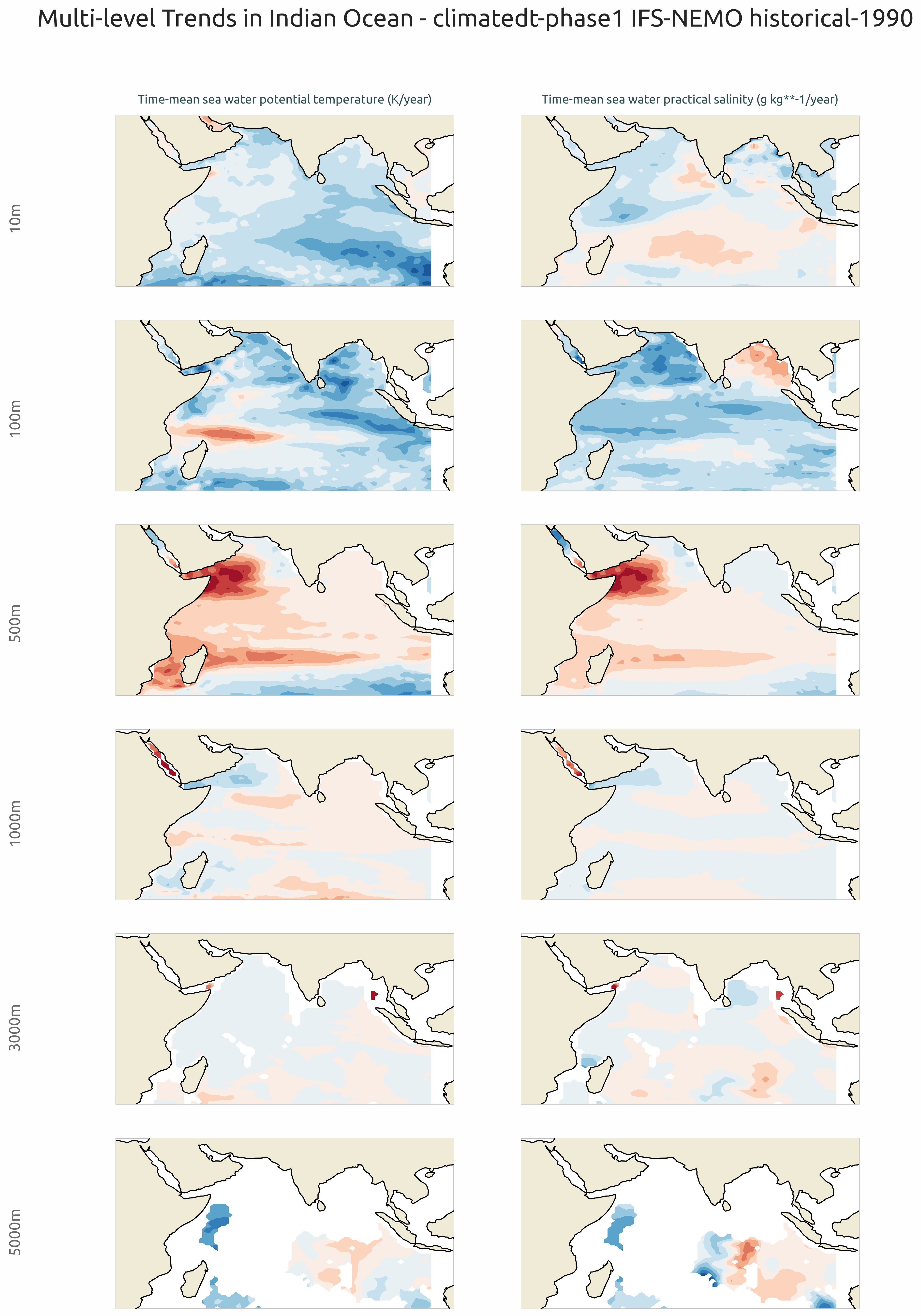
../_images/trends.multilevel_trend.climatedt-phase1.IFS-NEMO.historical-1990.r1.indian_ocean.png — Multi-level trend maps of sea water potential temperature and sea water practical salinity in the Indian Ocean. Rows show different depth levels (10m, 100m, 500m, 1000m, 3000m, 5000m). Positive values indicate warming trends.

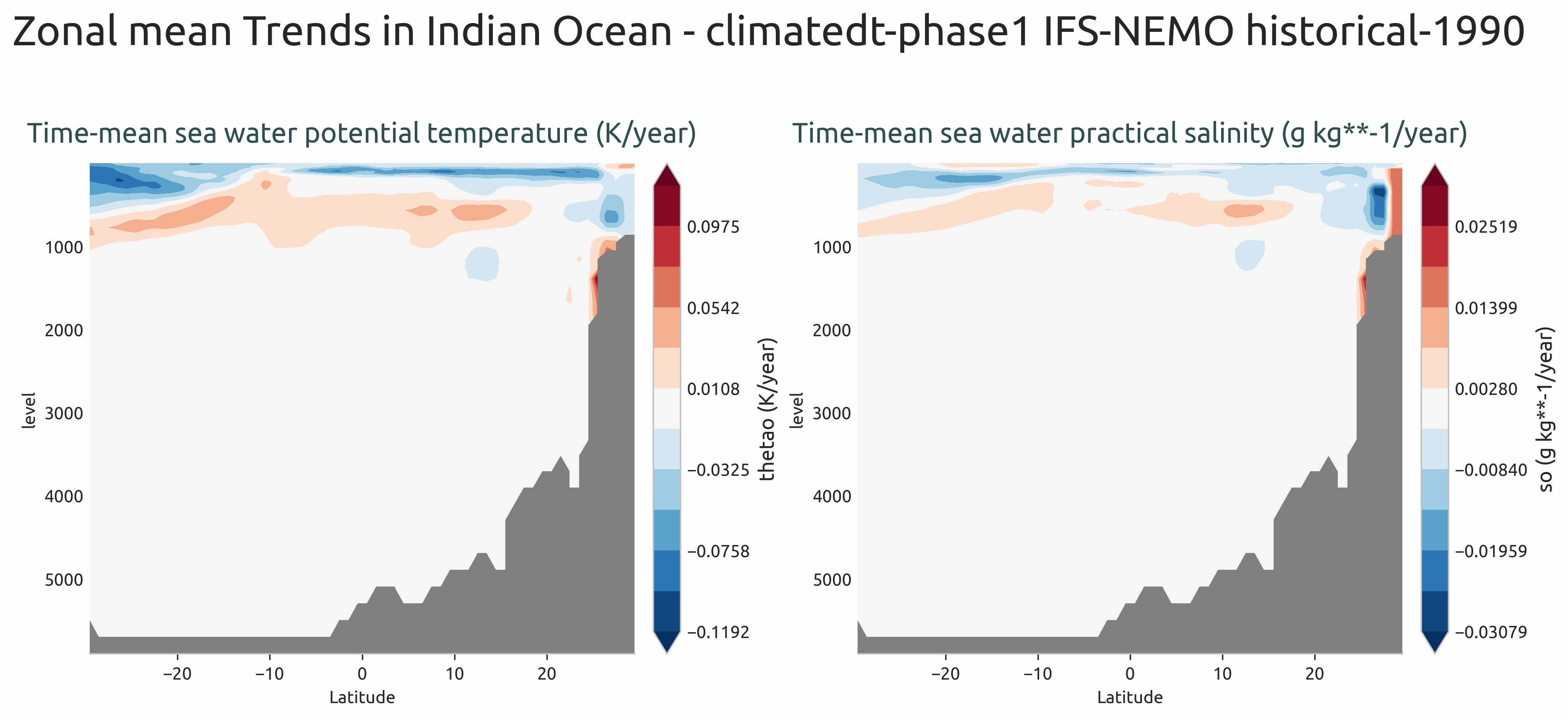
../_images/trends.zonal_mean.climatedt-phase1.IFS-NEMO.historical-1990.r1.indian_ocean.png — Zonal mean vertical section of potential temperature and practical salinity trends showing the meridional and depth structure.

Available demo notebooks

Notebooks are stored in notebooks/diagnostics/ocean_trends:

trends.ipynb

Authors and contributors

This diagnostic is maintained by Supriyo Gosh (@ghossh, supriyo.ghosh@bsc.es). Contributions are welcome — please open an issue or a pull request. For questions or suggestions, contact the AQUA team or the maintainer.

Detailed API

This section provides a detailed reference for the Application Programming Interface (API) of the “ocean3d” diagnostic, produced from the diagnostic function docstrings.

class aqua.diagnostics.ocean_trends.PlotTrends(data: Dataset, diagnostic_name: str = 'trends', vert_coord: str = 'level', outputdir: str = '.', rebuild: bool = True, loglevel: str = 'WARNING')

Bases: object

Class for plotting ocean trend diagnostics from xarray Datasets.

Class to plot trends from xarray Dataset.

Parameters:

data (xr.Dataset) – Input xarray Dataset containing trend data.
diagnostic_name (str, optional) – Name of the diagnostic for filenames. Defaults to “trends”.
vert_coord (str, optional) – Name of the vertical dimension coordinate. Defaults to DEFAULT_OCEAN_VERT_COORD.
outputdir (str, optional) – Directory to save output plots. Defaults to “.”.
rebuild (bool, optional) – Whether to rebuild output files. Defaults to True.
loglevel (str, optional) – Logging level. Default is “WARNING”.

plot_multilevel(levels: list = None, rebuild: bool = True, cbar_limits: dict = None, sym: bool = False, save_format: str | list = ['png', 'pdf', 'svg'], dpi: int = 300)

Plot multi-level maps of trends.

Parameters:

levels (list, optional) – List of depth levels to plot. Defaults to None.
rebuild (bool, optional) – If True, rebuild existing output files. Defaults to True.
cbar_limits (dict, optional) – Per-variable colorbar limits as {var: {‘vmin’: v, ‘vmax’: v}}. Defaults to None.
sym (bool, optional) – If True, use symmetric colorbar limits. Defaults to False.
save_format (str or list, optional) – Format(s) to save the figure in. Defaults to SAVE_FORMAT.
dpi (int, optional) – Resolution of the saved figure. Defaults to 300.

plot_zonal(rebuild: bool = True, save_format: str | list = ['png', 'pdf', 'svg'], dpi: int = 300)

Plot zonal mean vertical profiles of trends.

Parameters:

rebuild (bool, optional) – If True, rebuild existing output files. Defaults to True.
save_format (str or list, optional) – Format(s) to save the figure in. Defaults to SAVE_FORMAT.
dpi (int, optional) – Resolution of the saved figure. Defaults to 300.

save_plot(fig, diagnostic_product: str, extra_keys: dict = {}, rebuild: bool = True, dpi: int = 300, format: str | list = ['png', 'pdf', 'svg'], metadata: dict = None)

Save the plot to a file.

Parameters:

fig (matplotlib.figure.Figure) – The figure to be saved.
diagnostic_product (str) – The name of the diagnostic product. Default is None.
extra_keys (dict) – Extra keys to be used for the filename (e.g. season). Default is None.
rebuild (bool) – If True, the output files will be rebuilt. Default is True.
dpi (int) – The dpi of the figure. Default is 300.
format (str or list) – Format(s) to save the figure. Default is SAVE_FORMAT.
metadata (dict) – The metadata to be used for the figure. Default is None. They will be complemented with the metadata from the outputsaver. We usually want to add here the description of the figure.

set_cbar_labels(): Set the colorbar labels for each subplot from variable units.

set_central_longitude(): Set the central longitude for the map projection from the data.

set_data_list(): Prepare the list of data arrays to plot.

set_description(content=None): Set the description metadata for the plot.

set_extent(): Set the extent for the plot.

set_nrowcol(): Set the number of rows and columns for the subplot grid.

set_suptitle(plot_type=None): Set the title for the plot.

set_title(): Set the title for each subplot panel.

set_vmin_vmax(): Set per-variable colorbar min/max from cbar_limits if provided.

set_ytext(): Set the y-axis text for the multi-level plots.

class aqua.diagnostics.ocean_trends.Trends(model: str, exp: str, source: str, catalog: str = None, regrid: str = None, startdate: str = None, enddate: str = None, diagnostic_name: str = 'trends', vert_coord: str = 'level', loglevel: str = 'WARNING')

Bases: Diagnostic

Class to compute trends over time.

Initialize the Trends class.

Parameters:

model (str) – Climate model name.
exp (str) – Experiment name.
source (str) – Data source name.
catalog (str, optional) – Path to the data catalog.
regrid (str, optional) – Regridding method.
startdate (str, optional) – Start date for data selection.
enddate (str, optional) – End date for data selection.
diagnostic_name (str, optional) – Name of the diagnostic for filenames. Defaults to “trends”.
vert_coord (str, optional) – Name of the vertical dimension coordinate. Defaults to DEFAULT_OCEAN_VERT_COORD.
loglevel (str, optional) – Logging level. Default is “WARNING”.

MINIMUM_MONTHS_REQUIRED = 12

adjust_trend_for_time_frequency(trend, y_array)

Adjust trend values based on the time frequency of the data.

Parameters:

trend (xr.DataArray) – Trend values to adjust.
y_array (xr.DataArray) – Original data array with time coordinate.

Returns:

Adjusted trend values.

Return type:

xr.DataArray

compute_trend(data: DataArray | Dataset)

Compute linear trend coefficients over time.

Parameters:: data (xr.DataArray or xr.Dataset) – Input data with a time dimension.
Returns:: Trend coefficients adjusted for time frequency.
Return type:: xr.DataArray or xr.Dataset

run(outputdir: str = '.', rebuild: bool = True, region: str = None, var: list = ['thetao', 'so'], dim_mean: type = None, reader_kwargs: dict = {})

Run the trend analysis workflow.

Parameters:

outputdir (str, optional) – Directory to save output files. Default is current directory.
rebuild (bool, optional) – If True, rebuild existing files. Default is True.
region (str, optional) – Geographical region for analysis.
var (list, optional) – List of variable names to analyze. Default is [‘thetao’, ‘so’].
dim_mean (str or list, optional) – Dimension(s) over which to compute the mean. Default is None.
reader_kwargs (dict, optional) – Additional keyword arguments for the data reader. Default is {}.

save_netcdf(diagnostic_product: str = 'trend', outputdir: str = '.', rebuild: bool = True)

Save trend coefficients to a NetCDF file.

Parameters:

diagnostic (str, optional) – Diagnostic name for filenames. Default is “trends”.
diagnostic_product (str, optional) – Product type for filenames. Default is “spatial_trend”.
region (str, optional) – Geographical region for analysis.
outputdir (str, optional) – Directory to save output files. Default is current directory.
rebuild (bool, optional) – If True, rebuild existing files. Default is True.

select_region(data, region=None, drop=True, dim_mean=None)

Select a region and optionally compute mean over specified dimensions.

Parameters:

data (xr.Dataset) – Input dataset.
region (str, optional) – Geographical region to select.
drop (bool, optional) – Whether to drop coordinates outside the region. Default is True.
dim_mean (str or list, optional) – Dimension(s) over which to compute the mean.

Returns:

(data, region) - Processed data and region name.

Return type:

tuple