Ocean Drift Diagnostic
Description
The OceanDrift diagnostic is a set of tools for the analysis and visualization of temporal evolution and drift in ocean model outputs. It provides methods to assess model drift over time by analyzing Hovmöller diagrams and timeseries of ocean variables. The diagnostic supports analysis of full values, anomalies (relative to initial time or time mean), and standardized anomalies.
OceanDrift provides tools to:
Compute anomalies and standardized anomalies relative to the initial time (t0) or the time mean
Produce timeseries plots at specific depth levels
Generate Hovmöller diagrams showing the temporal evolution of ocean variables as a function of depth
Perform spatial averaging over predefined ocean regions (e.g., Atlantic Ocean, Pacific Ocean, Global Ocean)
Classes
There are two main classes for analysis and plotting:
Hovmoller: retrieves ocean data (typically temperature and salinity) and processes it for drift analysis. It handles spatial averaging over specified regions and computation of anomalies and standardized anomalies. The diagnostic supports different reference types for anomaly computation:
t0: Anomalies computed relative to the first time step (initial state)tmean: Anomalies computed relative to the time mean of the entire periodNone: No anomaly computation (full values only)
PlotHovmoller: provides methods for plotting Hovmöller diagrams and timeseries. It generates multi-panel plots showing different anomaly types and variables.
File structure
The diagnostic is located in the
aqua/diagnostics/ocean_driftdirectory, which contains both the source code and the command line interface (CLI) script.A template configuration file is available at
aqua/diagnostics/templates/diagnostics/config-ocean_drift.yamlNotebooks are available in the
notebooks/diagnostics/ocean_driftdirectory and contain examples of how to use the diagnostic.Regions definitions are available in
aqua/diagnostics/config/tools/ocean3d/definitions/regions.yaml
Input variables and datasets
The diagnostic works with 3D ocean model outputs and can be applied to any ocean variable.
The primary variables typically used in this diagnostic are:
thetao(sea water potential temperature)so(sea water salinity)
The diagnostic is designed to work with data from the Low Resolution Archive (LRA), generated by the Data reduction OPerator (DROP) of the AQUA project, which provides monthly data at a 1x1 degree resolution. A higher resolution is not necessary for this diagnostic.
Basic usage
The basic usage of this diagnostic is explained with a working example in the notebook. The basic structure of the analysis is the following:
from aqua.diagnostics import Hovmoller, PlotHovmoller

hov = Hovmoller(
    catalog='climatedt-phase1',
    model='IFS-NEMO',
    exp='historical-1990',
    source='lra-r100-monthly',
    startdate='01-01-1991',
    enddate='31-05-1991',
    loglevel='INFO'
)


hov.run(
    region='io',
    dim_mean=['lat', 'lon'],
    anomaly_ref='t0'
)

hov_plot = PlotHovmoller(data=hov.processed_data_list)
hov_plot.plot_hovmoller()
hov_plot.plot_timeseries()
Note
The diagnostic automatically processes data to generate all transformation types (full values, anomalies and standardized anomalies). Spatial averaging is performed over the specified dimensions before computing temporal transformations.
CLI usage
The diagnostic can be run from the command line interface (CLI) by running the following command:
cd $AQUA/aqua/diagnostics/ocean_drift
python cli_ocean_drift.py --config <path_to_config_file>
Additionally, the CLI can be run with the following optional arguments:
--config,-c: Path to the configuration file.--nworkers,-n: Number of workers to use for parallel processing.--cluster: Cluster to use for parallel processing. By default a local cluster is used.--loglevel,-l: Logging level. Default isWARNING.--catalog: Catalog to use for the analysis. Can be defined in the config file.--model: Model to analyse. Can be defined in the config file.--exp: Experiment to analyse. Can be defined in the config file.--source: Source to analyse. Can be defined in the config file.--outputdir: Output directory for the plots.--startdate: Start date for the analysis.--enddate: End date for the analysis.
Configuration file structure
The configuration file is a YAML file that contains the details on the dataset to analyse, the output directory and the diagnostic settings. Most of the settings are common to all the diagnostics (see Diagnostics configuration files). Here we describe only the specific settings for the ocean drift diagnostic.
ocean_drift: a block (nested in thediagnosticsblock) containing options for the Ocean Drift diagnostic.hovmoller: sub-block containing specific parameters for Hovmöller analysis.run: enable/disable the diagnostic.diagnostic_name: name of the diagnostic.ocean3dby default.vert_coord: vertical coordinate for the analysis (e.g.,level).var: list of variables to analyse (typically['thetao', 'so']).regions: list of ocean regions to analyse (e.g.,['go', 'io', 'ao', 'so', 'arc_o', 'po']).dim_mean: dimensions over which to compute spatial averages (typically['lat', 'lon']).
diagnostics:
  ocean_drift:
    hovmoller:
      diagnostic_name: 'ocean3d'
      vert_coord: level
      run: true
      var: ['thetao', 'so']
      regions: ['io', 'sss']
      dim_mean: ['lat', 'lon']
The diagnostic supports analysis over predefined ocean regions. Common regions include:
io- Indian Oceanao- Atlantic Oceanpo- Pacific Oceanarc_o- Arctic Oceango- Global Oceanss- Sargasso Sea
Additional regions can be defined in aqua/diagnostics/config/tools/ocean3d/definitions/regions.yaml.
Output
The diagnostic produces two types of plots:
Hovmöller diagrams showing the temporal evolution of ocean variables as a function of depth, with separate panels for each transformation type (full values, anomalies, standardized anomalies)
Timeseries plots showing the temporal evolution at specific depth levels, with multiple lines representing different depths
If not specified otherwise, plots will be saved both in PNG and PDF format. Data outputs (containing the computed anomalies over the specified regions) are saved as NetCDF files for further analysis.
Example Plots
All plots can be reproduced using the notebooks in the notebooks directory on LUMI HPC.
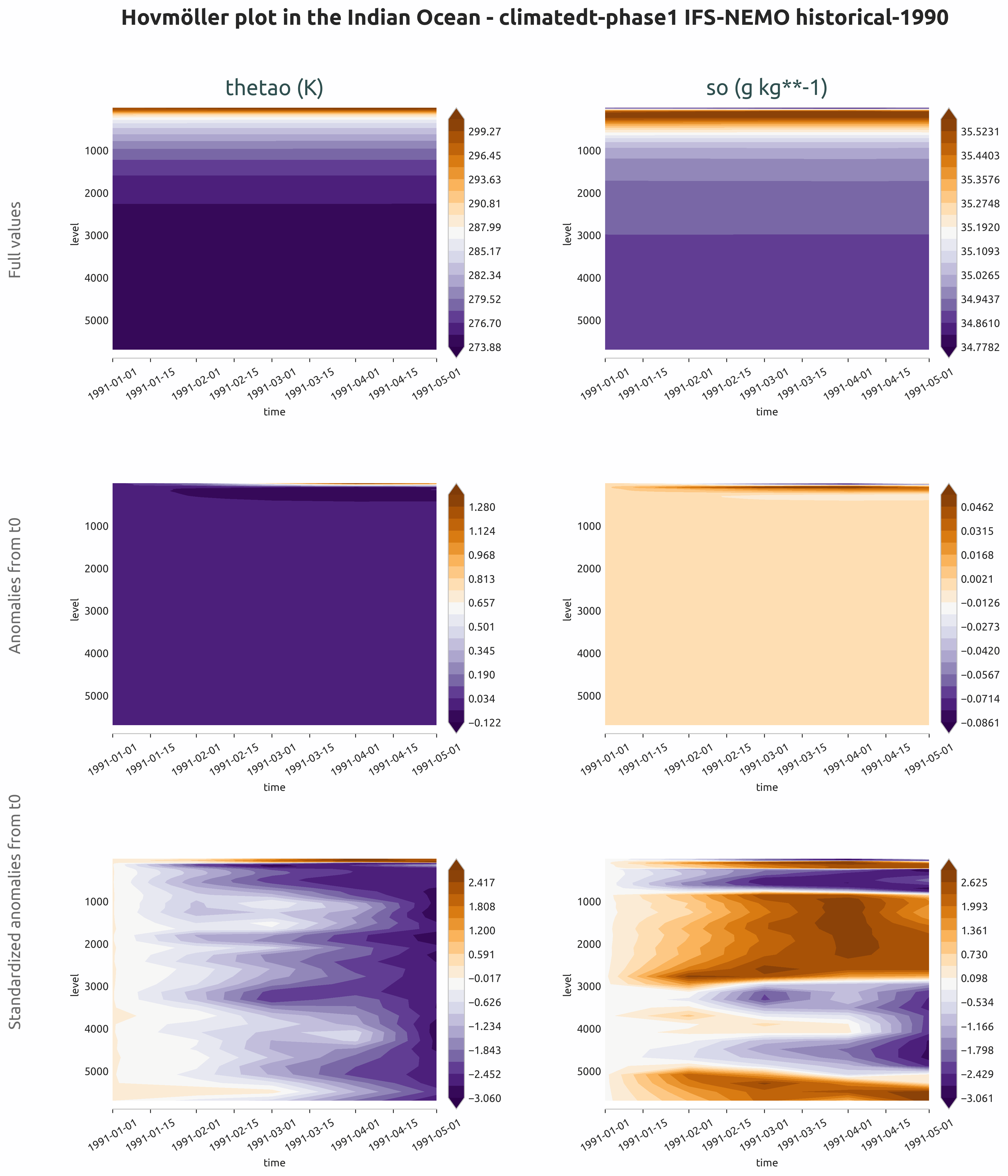
Hovmöller diagrams showing ocean temperature drift in the Indian Ocean. Full values, anomalies relative to initial time and standardized anomalies are shown.
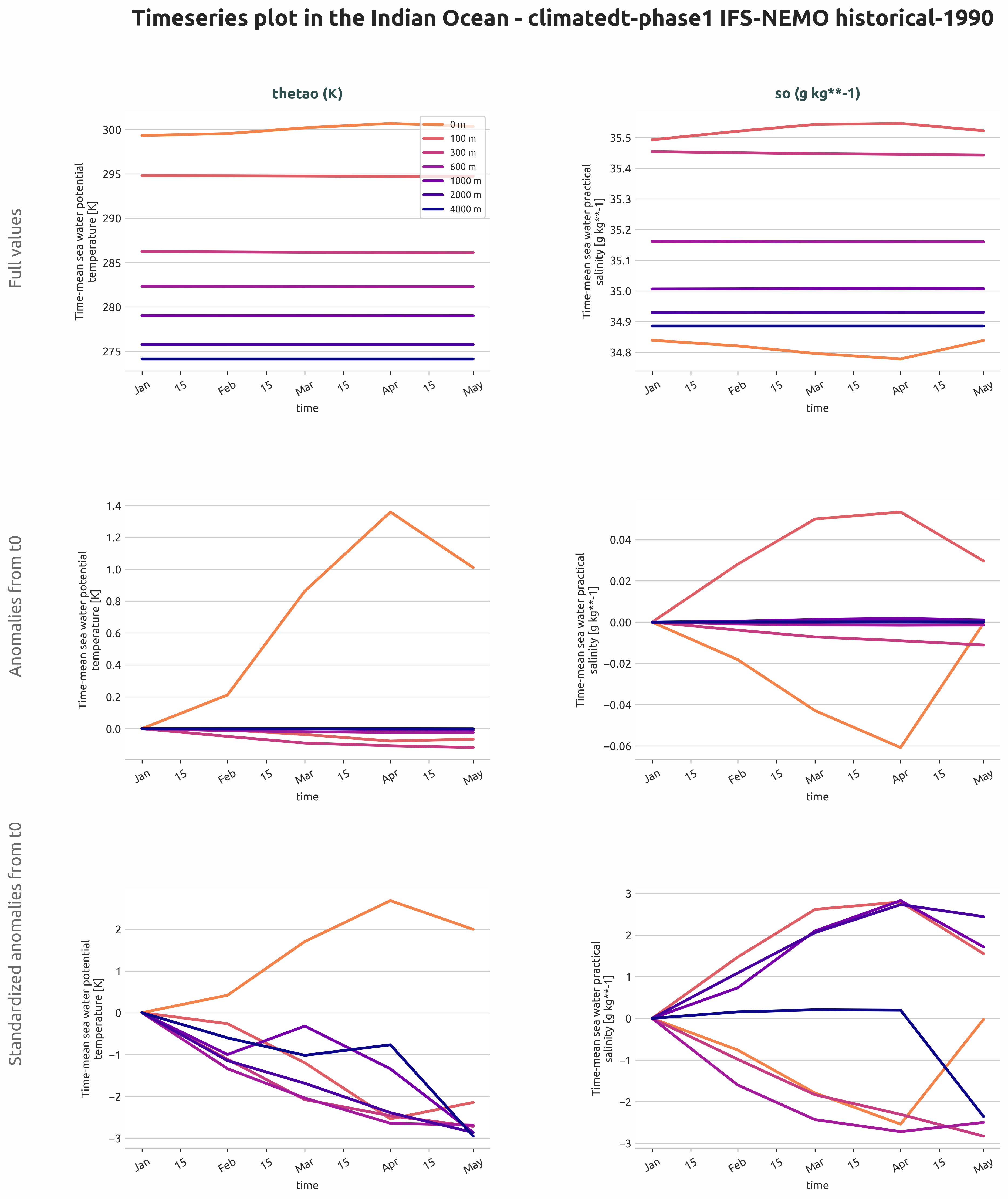
Timeseries of ocean temperature at multiple depth levels in the Indian Ocean, showing drift patterns from full values, anomalies relative to t0, and standardized anomalies.
Available demo notebooks
Notebooks are stored in notebooks/diagnostics/ocean_drift:
Detailed API
This section provides a detailed reference for the Application Programming Interface (API) of the Ocean_drift diagnostic,
produced from the diagnostic function docstrings.
- class aqua.diagnostics.ocean_drift.Hovmoller(model: str, exp: str, source: str, catalog: str = None, regrid: str = None, startdate: str = None, enddate: str = None, diagnostic_name: str = 'oceandrift', vert_coord: str = 'depth', loglevel: str = 'WARNING')
Bases:
DiagnosticA class for generating Hovmoller diagrams from ocean model data.
This class provides methods to retrieve, process, and save netCDF files for Hovmoller diagrams. It inherits from the Diagnostic class.
- logger
Logger instance for the class.
- Type:
Logger
- outputdir
Directory to save the output files.
- Type:
str
- region
Region for area selection.
- Type:
str
- var
List of variables to process.
- Type:
list
- stacked_data
Processed data for Hovmoller diagrams.
- Type:
xarray.Dataset
Initialize the Hovmoller class.
- Parameters:
model (str) – Model name.
exp (str) – Experiment name.
source (str) – Data source.
catalog (str, optional) – Path to the catalog file.
regrid (str, optional) – Regridding method.
startdate (str, optional) – Start date for data retrieval.
enddate (str, optional) – End date for data retrieval.
diagnostic_name (str, optional) – Name of the diagnostic for filenames. Defaults to “oceandrift”.
vert_coord (str, optional) – Name of the vertical dimension coordinate. Defaults to DEFAULT_OCEAN_VERT_COORD.
loglevel (str, optional) – Logging level. Defaults to “WARNING”.
- MINIMUM_MONTHS_REQUIRED = 2
- compute_hovmoller(dim_mean: str = None, anomaly_ref: str | list = None)
Process input data for drift analysis by applying various transformations and aggregations.
- Parameters:
dim_mean (str or None) – The dimension along which to compute the mean. If None, no mean is computed.
anomaly_ref (str or list, optional) – Reference for anomaly calculation. Can be “t0”, “tmean”, or None. By default, full values are used.
- Returns:
A concatenated DataArray containing processed data for different combinations of anomaly, standardization, and anomaly reference types.
- Return type:
xarray.DataArray
- run(outputdir: str = '.', rebuild: bool = True, region: str = None, var: list = ['thetao', 'so'], dim_mean=['lat', 'lon'], anomaly_ref: str = None, reader_kwargs: dict = {})
Run the Hovmoller diagram generation workflow.
This method retrieves the specified variables, applies region selection if provided, computes Hovmoller diagrams with optional mean and anomaly processing, and saves the results to netCDF files.
- Parameters:
outputdir (str, optional) – Directory to save the output files. Defaults to “.”.
rebuild (bool, optional) – Whether to rebuild the netCDF file. Defaults to True.
region (str, optional) – Region for area selection. Defaults to None (global evaluation).
var (list, optional) – List of variables to process. Defaults to [“thetao”, “so”].
dim_mean (list, optional) – List of dimensions over which to compute the mean. Defaults to [“lat”, “lon”].
anomaly_ref (str or None, optional) – Reference for anomaly calculation. Can be “t0”, “tmean”, or None.
reader_kwargs (dict, optional) – Additional keyword arguments for the Reader. Defaults to {}.
- save_netcdf(diagnostic_product: str = 'hovmoller', region: str = None, outputdir: str = '.', rebuild: bool = True)
Save the processed data to a netCDF file.
- Parameters:
diagnostic_product (str) – Name of the diagnostic product.
region (str) – Region for area selection. Defaults to None.
outputdir (str) – Directory to save the output files. Defaults to ‘.’.
rebuild (bool, optional) – Whether to rebuild the netCDF file. Defaults to True.
- sort_key(data)
Return a sort key for ordering processed data by drift type.
- class aqua.diagnostics.ocean_drift.PlotHovmoller(data: list[Dataset], diagnostic_name: str = 'oceandrift', vert_coord: str = 'depth', outputdir: str = '.', loglevel: str = 'WARNING')
Bases:
objectClass for plotting Hovmoller diagrams and timeseries from AQUA ocean drift diagnostics.
This class provides methods to generate, customize, and save Hovmoller and timeseries plots using xarray datasets and AQUA conventions. It handles metadata extraction, plot styling, and output file management.
Initialize the PlotHovmoller class.
- Parameters:
data (list[xr.Dataset]) – List of xarray datasets containing the data to be plotted
diagnostic_name (str) – Name of the diagnostic, default is “oceandrift”
vert_coord (str) – Name of the vertical dimension coordinate, default is “level”
outputdir (str) – Directory where the output will be saved, default is current directory
loglevel (str) – Logging level, default is “WARNING”
- plot_hovmoller(rebuild: bool = True, save_format: list = ['png', 'pdf', 'svg'], dpi: int = 300)
Plot the Hovmoller diagram for the given data.
This method sets the title, description, vmax, vmin, and texts for the plot. It then calls the plot_multi_hovmoller function to create the plot and saves it using the OutputSaver.
- Parameters:
rebuild (bool) – Whether to rebuild the output, default is True.
save_format (str or list) – List of formats to save the figure. Default is SAVE_FORMAT.
dpi (int) – Dots per inch for the saved figure. Default is 300.
- Returns:
None
- plot_timeseries(levels: list = None, rebuild: bool = True, save_format: list = ['png', 'pdf', 'svg'], dpi: int = 300)
Plot the timeseries for the given data.
This method sets the title, description, vmax, vmin, and texts for the plot. It then calls the plot_multi_timeseries function to create the plot and saves it using the OutputSaver.
- Parameters:
levels (list, optional) – List of levels to plot. Default is None.
rebuild (bool) – Whether to rebuild the output, default is True.
save_format (list) – List of formats to save the figure. Default is SAVE_FORMAT.
dpi (int) – Dots per inch for the saved figure. Default is 300.
- Returns:
None
- save_plot(fig, diagnostic_product: str = None, extra_keys: dict = None, metadata: dict = None, rebuild: bool = True, dpi: int = 300, format: str = ['png', 'pdf', 'svg'])
Save the plot to a file.
- Parameters:
fig (matplotlib.figure.Figure) – The figure to be saved.
diagnostic_product (str) – The name of the diagnostic product. Default is None.
extra_keys (dict) – Extra keys to be used for the filename (e.g. season). Default is None.
rebuild (bool) – If True, the output files will be rebuilt. Default is True.
dpi (int) – The dpi of the figure. Default is 300.
format (str or list) – Format(s) to save the figure. Default is SAVE_FORMAT.
metadata (dict) – The metadata to be used for the figure. Default is None. They will be complemented with the metadata from the outputsaver. We usually want to add here the description of the figure.
- set_data_for_levels()
Extract and set the data at the specified depth levels.
- set_data_type()
Set the data type list for each dataset based on its AQUA attributes.
- set_description(content: str = None)
Set the description for the Hovmoller plot.
- set_levels()
Set the levels and corresponding labels for timeseries plots.
- set_line_plot_colours()
Set the color list for line plots based on the number of levels.
- set_suptitle(content: str = None)
Set the suptitle for the Hovmoller plot.
- set_texts()
Set the text annotations for each subplot panel based on drift type.
- set_title()
Set the title for each subplot panel.
- set_vmax_vmin()
Set the vmax, vmin, and colormap for each subplot from the data type.