Teleconnections Diagnostic
Description
The teleconnections diagnostic is a set of tools to compute the most relevant teleconnections. NAO (North Atlantic Oscillation), ENSO (El Niño Southern Oscillation) and MJO (Madden-Julian Oscillation) are the teleconnections currently implemented. The diagnostic is built to evaluate the teleconnections indices and to compute regression and correlation maps with respect to the teleconnection index.
Note
MJO is currently missing a command line interface and it is not operational yet.
Classes
There are three classes for the analysis:
NAO: computes the NAO index based on mean sea level pressure (msl) using the station-based method, and computes regression and correlation maps with respect to the NAO index.
ENSO: computes the ENSO index based on sea surface temperature (tos) using the Niño3.4 region, and computes regression and correlation maps with respect to the ENSO index.
MJO: computes the MJO Hovmoeller plots based on the top net thermal radiation flux (tnlwrf) variable.
There are three other classes for the plots:
PlotNAO: produces the NAO index time series and the regression and correlation maps.
PlotENSO: produces the ENSO index time series and the regression and correlation maps.
PlotMJO: produces the MJO Hovmoeller plots.
File structure
The diagnostic is located in the
aqua/diagnostics/teleconnectionsdirectory, which contains the source code and the command line interface (CLI) script.A template configuration file is available at
aqua/diagnostics/templates/diagnostics/config-teleconnections.yamlNotebooks are available in the
notebooks/diagnostics/teleconnectionsdirectory and contain examples of how to use the diagnostic.Interface files to specify custom regions or other variable names for the index evaluation are available in the
aqua/diagnostics/config/tools/teleconnections/definitionsdirectory.
Note
A command line to evaluate, using the bootstrap method, the concordance maps of regression and correlation is available in the cli_bootstrap.py file.
This is not included in any automatic run of the diagnostic because it is a time-consuming process.
Please note that the bootstrap CLI is not actively maintained and has not yet been tested against recent API changes or imports.
Input variables and datasets
By default, the diagnostic compares against the ERA5 dataset, with the index evaluated over the entire available period (1940 to present).
The necessary variables for the default evaluation are:
msl(mean sea level pressure) for NAOtos(sea surface temperature) for ENSOtnlwrf(top net thermal radiation flux) for MJO
Other variables can be used for the regression and correlation maps.
The diagnostic is designed to work with data from the Low Resolution Archive (LRA), generated by the Data Reduction OPerator (DROP) of the AQUA project, which provides monthly data at a 1x1 degree resolution.
Basic usage
The basic usage of this diagnostic is explained with working examples in the notebooks. The basic structure of the analysis is the following:
from aqua.diagnostics import NAO, PlotNAO

nao_dataset = NAO(
    catalog='climatedt-phase1',
    model='IFS-NEMO',
    exp='historical-1990',
    source='lra-r100-monthly',
    loglevel=loglevel)

nao_obs = NAO(
    catalog='obs',
    model='ERA5',
    exp='era5',
    source='monthly',
    loglevel=loglevel)

nao_dataset.retrieve()
nao_obs.retrieve()

nao_dataset.compute_index()
nao_obs.compute_index()

reg_dataset = nao_dataset.compute_regression(season='DJF')
reg_obs = nao_obs.compute_regression(season='DJF')

plot = PlotNAO(loglevel='INFO', indexes=nao_dataset.index,
           ref_indexes=nao_obs.index)

fig_index, _ = plot.plot_index()
Note
Start/end dates and reference dataset can be customized. If not specified otherwise, plots will be saved in PNG and PDF format in the current working directory.
CLI usage
The diagnostic can be run from the command line interface (CLI) by running the following command:
cd $AQUA/aqua/diagnostics/teleconnections
python cli_teleconnections.py --config <path_to_config_file>
Three configuration files are provided and run when executing the aqua-analysis (see AQUA analysis wrapper). Two configuration files are for atmospheric and oceanic teleconnections.
Additionally, the CLI can be run with the following optional arguments:
--config,-c: Path to the configuration file.--nworkers,-n: Number of workers to use for parallel processing.--cluster: Cluster to use for parallel processing. By default a local cluster is used.--loglevel,-l: Logging level. Default isWARNING.--catalog: Catalog to use for the analysis. Can be defined in the config file.--model: Model to analyse. Can be defined in the config file.--exp: Experiment to analyse. Can be defined in the config file.--source: Source to analyse. Can be defined in the config file.--outputdir: Output directory for the plots.--startdate: Start date for the analysis.--enddate: End date for the analysis.
Configuration file structure
The configuration file is a YAML file that contains the details on the dataset to analyse or use as reference, the output directory and the diagnostic settings. Most of the settings are common to all the diagnostics (see Diagnostics configuration files). Here we describe only the specific settings for the teleconnections diagnostic.
teleconnections: a block (nested in thediagnosticsblock), containing options for the teleconnections.It allows to specify which teleconnections to run, the months window for the rolling mean, the seasons to consider, and the color bar range for the plots. It contains the following blocks:
NAO: a block, nested in theteleconnectionsblock, that contains the details required for the NAO teleconnection.ENSO: a block, nested in theteleconnectionsblock, that contains the details required for the ENSO teleconnection.
diagnostics:
    teleconnections:
        NAO:
            run: true
            diagnostic_name: 'nao'
            months_window: 3
            seasons: ['DJF']
            cbar_range: [-5, 5]
        ENSO:
            run: true
            diagnostic_name: 'enso'
            months_window: 3
            seasons: ['annual']
            cbar_range: [-2, 2]
Output
The diagnostic produces the following outputs:
NAO: North Atlantic Oscillation index, regression and correlation maps.
ENSO: El Niño Southern Oscillation index, regression and correlation maps.
MJO: Madden-Julian Oscillation Hovmoeller plots of the Mean top net thermal radiation flux variable.
Plots are saved in both PDF and PNG format. Data outputs are saved as NetCDF files.
If a reference dataset is provided, the automatic maps consist of contour lines for the model regression map and filled contour map for the difference between the model and the reference regression map.
Observations
The default reference dataset is ERA5 reanalysis, provided by ECMWF.
The diagnostic uses ERA5 monthly averages from the AQUA obs catalog (model=ERA5, exp=era5, source=monthly).
Custom reference datasets can be configured in the configuration file.
Example Plots
All plots can be reproduced using the notebooks in the notebooks directory on LUMI HPC.
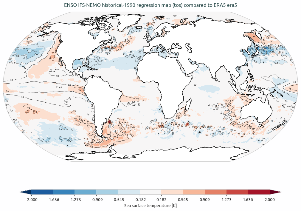
ENSO IFS-NEMO ssp370 regression map (avg_tos) compared to ERA5. The contour lines are the model regression map and the filled contour map is the difference between the model and the reference regression map (ERA5).
Available demo notebooks
Notebooks are stored in notebooks/diagnostics/teleconnections:
Detailed API
This section provides a detailed reference for the Application Programming Interface (API) of the teleconnections diagnostic,
produced from the diagnostic function docstrings.
Teleconnections module
- class aqua.diagnostics.teleconnections.ENSO(catalog: str = None, model: str = None, exp: str = None, source: str = None, regrid: str = None, startdate: str = None, enddate: str = None, configdir: str = None, definition: str = 'teleconnections-destine', loglevel: str = 'WARNING')
Bases:
BaseMixinClass for calculating the El Niño Southern Oscillation (ENSO) index. This class is used to calculate the ENSO index from a given dataset. It inherits from the BaseMixin class and implements the necessary methods to calculate the ENSO index.
Initialize the ENSO class.
- Parameters:
catalog (str) – Catalog name.
model (str) – Model name.
exp (str) – Experiment name.
source (str) – Source name.
regrid (str) – Regrid target. Default is None.
startdate (str) – Start date for data retrieval. Default is None.
enddate (str) – End date for data retrieval. Default is None.
configdir (str) – Configuration directory. Default is None.
definition (str) – definition filename. Default is ‘teleconnections-destine’. This is used to deduce the variable name and the lat/lon for the index.
loglevel (str) – Logging level. Default is ‘WARNING’.
- MINIMUM_MONTHS_REQUIRED = 24
- compute_index(months_window: int = 3, box_brd: bool = True, rebuild: bool = False)
” Evaluate station based index for a teleconnection. Field data must be monthly gridded data.
- Parameters:
months_window (int, opt) – months for rolling average, default is 3
box_brd (bool, opt) – choose if coordinates are comprised or not. Default is True
rebuild (bool, opt) – if True, the index is recalculated, default is False
- retrieve(reader_kwargs: dict = {}) None
Retrieve the data for the ENSO index.
- Parameters:
reader_kwargs (dict) – Additional keyword arguments for the Reader. Default is an empty dictionary.
- class aqua.diagnostics.teleconnections.MJO(catalog: str = None, model: str = None, exp: str = None, source: str = None, regrid: str = None, startdate: str = None, enddate: str = None, configdir: str = None, definition: str = 'teleconnections-destine', loglevel: str = 'WARNING')
Bases:
BaseMixinMJO (Madden-Julian Oscillation) class.
Initialize the MJO class.
- Parameters:
catalog (str) – Catalog name.
model (str) – Model name.
exp (str) – Experiment name.
source (str) – Source name.
regrid (str) – Regrid method.
startdate (str) – Start date for data retrieval.
enddate (str) – End date for data retrieval.
configdir (str) – Configuration directory. Default is the installation directory.
definition (str) – definition filename. Default is ‘teleconnections-destine’.
loglevel (str) – Logging level. Default is ‘WARNING’.
- MINIMUM_MONTHS_REQUIRED = 24
- compute_hovmoller(day_window: int = None)
Compute the Hovmoller plot for the MJO index. This method prepares the data for a Hovmoller plot by selecting the MJO box, evaluating anomalies, and smoothing the data if required.
- Parameters:
day_window (int, optional) – Number of days to be used in the smoothing window. If None, no smoothing is performed. Default is None.
- retrieve(reader_kwargs: dict = {}) None
Retrieve the data for the MJO Hovmoller plot.
- Parameters:
reader_kwargs (dict) – Additional keyword arguments for the Reader. Default is an empty dictionary.
- class aqua.diagnostics.teleconnections.NAO(catalog: str = None, model: str = None, exp: str = None, source: str = None, regrid: str = None, startdate: str = None, enddate: str = None, configdir: str = None, definition: str = 'teleconnections-destine', loglevel: str = 'WARNING')
Bases:
BaseMixinNorth Atlantic Oscillation (NAO) index calculation class. This class is used to calculate the NAO index from a given dataset. It inherits from the BaseMixin class and implements the necessary methods to calculate the NAO index.
Initialize the NAO class.
- Parameters:
catalog (str) – Catalog name.
model (str) – Model name.
exp (str) – Experiment name.
source (str) – Source name.
regrid (str) – Regrid method.
startdate (str) – Start date for data retrieval.
enddate (str) – End date for data retrieval.
configdir (str) – Configuration directory. Default is the installation directory.
definition (str) – definition filename. Default is ‘teleconnections-destine’.
loglevel (str) – Logging level. Default is ‘WARNING’.
- MINIMUM_MONTHS_REQUIRED = 24
- compute_index(months_window: int = 3, rebuild: bool = False)
” Evaluate station based index for a teleconnection. Field data must be monthly gridded data.
- Parameters:
months_window (int, opt) – months for rolling average, default is 3
rebuild (bool, opt) – if True, the index is recalculated, default is False
- retrieve(reader_kwargs: dict = {}) None
Retrieve the data for the NAO index.
- Parameters:
reader_kwargs (dict) – Additional keyword arguments for the Reader. Default is an empty dictionary.
- class aqua.diagnostics.teleconnections.PlotENSO(indexes=None, ref_indexes=None, outputdir: str = './', rebuild: bool = True, loglevel: str = 'WARNING')
Bases:
PlotBaseMixinPlot the ENSO products.
- Parameters:
indexes (list) – List of indexes to plot.
ref_indexes (list) – List of reference indexes to plot.
outputdir (str) – Directory to save the plots. Default is ‘./’.
rebuild (bool) – If True, rebuild the plots. Default is True.
loglevel (str) – Log level for the logger. Default is ‘WARNING’.
- plot_index(thresh: float = 0.5, labels: list = None)
Plot the indexes for the ENSO products.
- Parameters:
thresh (float) – Threshold for the indexes. Default is 0.5.
labels (list) – List of labels for the indexes. Default is None, in this case labels will be set by the set_labels method.
- Returns:
Figure object. axs: Axes object.
- Return type:
fig
- plot_maps(maps=None, ref_maps=None, statistic: str = None, vmin: float = None, vmax: float = None, vmin_diff: float = None, vmax_diff: float = None, **kwargs)
Plot the maps for the ENSO products.
- Parameters:
maps (list) – List of maps to plot.
ref_maps (list) – List of reference maps to plot.
statistic (str) – Statistic to plot. Default is None.
vmin (float) – Minimum value for the color value. Default is None.
vmax (float) – Maximum value for the color value. Default is None.
vmin_diff (float) – Minimum value for the color value for the difference. Default is None.
vmax_diff (float) – Maximum value for the color value for the difference. Default is None.
**kwargs – Additional arguments for the plotting function.
- Returns:
Figure object.
- Return type:
fig
- set_index_description()
Set the description of the index. This is used to generate the caption of the figure.
- Parameters:
index_name (str) – The name of the index. Default is None.
- Returns:
The caption of the figure.
- Return type:
str
- set_map_description(maps=None, ref_maps=None, statistic: str = None)
Set the description for the maps.
- Parameters:
maps (list) – List of maps to plot.
ref_maps (list) – List of reference maps to plot.
statistic (str) – Statistic to plot. Default is None.
- Returns:
Description of the maps.
- Return type:
str
- class aqua.diagnostics.teleconnections.PlotMJO(data, outputdir: str = './', loglevel: str = 'WARNING')
Bases:
objectPlotMJO class for plotting the MJO Hovmoller data. This class is a placeholder for future plotting methods.
Initialize the PlotMJO class.
- Parameters:
data (xarray.DataArray) – Data to be plot.
outputdir (str) – Directory where the plots will be saved. Default is ‘./’.
loglevel (str) – Logging level. Default is ‘WARNING’.
- plot_hovmoller(invert_axis: bool = True, invert_time: bool = True, nlevels: int = 21, cmap: str = 'PuOr', vmin: float = -90, vmax: float = 90)
Plot the Hovmoller diagram for the MJO data.
- Parameters:
invert_axis (bool) – If True, invert the axis. Default is True.
invert_time (bool) – If True, invert the time axis. Default is True.
nlevels (int) – Number of contour levels. Default is 21.
cmap (str) – Colormap to use for the plot. Default is ‘PuOr’.
vmin (float) – Minimum value for the colorbar. Default is -90.
vmax (float) – Maximum value for the colorbar. Default is 90.
- Returns:
The Hovmoller plot figure.
- Return type:
fig (matplotlib.figure.Figure)
- save_plot(fig, diagnostic_product: str = 'hovmoller', extra_keys: dict = None, rebuild: bool = True, metadata: dict = None, format: str | list = ['png', 'pdf', 'svg'], dpi: int = 300)
Save the plot to a file.
- Parameters:
fig (matplotlib.figure.Figure) – The figure to be saved.
diagnostic_product (str) – The name of the diagnostic product. Default is None.
extra_keys (dict) – Extra keys to be used for the filename (e.g. season). Default is None.
rebuild (bool) – If True, the output files will be rebuilt. Default is True.
dpi (int) – The dpi of the figure. Default is 300.
format (str or list) – Format(s) to save the figure. Default is SAVE_FORMAT.
metadata (dict) – The metadata to be used for the figure. Default is None. They will be complemented with the metadata from the outputsaver. We usually want to add here the description of the figure.
- class aqua.diagnostics.teleconnections.PlotNAO(indexes=None, ref_indexes=None, outputdir: str = './', rebuild: bool = True, loglevel: str = 'WARNING')
Bases:
PlotBaseMixinPlot the NAO products.
- Parameters:
indexes (list) – List of indexes to plot.
ref_indexes (list) – List of reference indexes to plot.
outputdir (str) – Directory to save the plots. Default is ‘./’.
rebuild (bool) – If True, rebuild the plots. Default is True.
loglevel (str) – Log level for the logger. Default is ‘WARNING’.
- plot_index(thresh: float = 0.0, labels: list = None)
Plot the NAO index.
- Parameters:
thresh (float) – Threshold for the index. Default is 0.0.
labels (list) – List of labels for the indexes. Default is None, in which case the labels are set automatically.
- Returns:
Figure object. axs: Axes object.
- Return type:
fig
- plot_maps(maps=None, ref_maps=None, statistic: str = None, vmin: float = None, vmax: float = None, vmin_diff: float = None, vmax_diff: float = None, **kwargs)
Plot the maps for the NAO products.
- Parameters:
maps (list) – List of maps to plot.
ref_maps (list) – List of reference maps to plot.
statistic (str) – Statistic to plot. Default is None.
vmin (float) – Minimum value for the color value. Default is None.
vmax (float) – Maximum value for the color value. Default is None.
vmin_diff (float) – Minimum value for the color value for the difference. Default is None.
vmax_diff (float) – Maximum value for the color value for the difference. Default is None.
**kwargs – Additional arguments for the plotting function.
- Returns:
Figure object.
- Return type:
fig
- set_index_description()
Build the description for the NAO index plot. Adds information about the months window used to compute the index.
- set_map_description(maps=None, ref_maps=None, statistic: str = None)
Set the description for the maps.
- Parameters:
maps (list) – List of maps to plot.
ref_maps (list) – List of reference maps to plot.
statistic (str) – Statistic to plot. Default is None.
- Returns:
Description of the maps.
- Return type:
str