Ensemble Zonal diagnostic

Description

The EnsembleZonal diagnostic provides tools to compute and visualize ensemble statistics of zonal-mean level-latitude cross-sections:

• Compute ensemble mean and standard deviation for zonal-mean cross-sections

• Generate contour plots showing ensemble statistics as functions of latitude and depth/level

Classes

There is one class for the analysis and one for the plotting:

• EnsembleZonal: computes ensemble mean and standard deviation for zonal-mean level-latitude cross-sections. Results are saved as class attributes and as NetCDF files.

• PlotEnsembleZonal: provides methods for plotting zonal cross-sections of ensemble mean and standard deviation.

File structure

• The diagnostic is located in the aqua/diagnostics/ensemble directory, which contains both the source code and the command line interface (CLI) scripts.

• Template configuration files are available in the aqua/diagnostics/templates/diagnostics/config-ensemble_zonalmean.yaml directory.

• Notebooks are available in the notebooks/diagnostics/ensemble directory and contain examples of how to use the diagnostic.

Input variables and datasets

Before using the diagnostic, input data must be loaded and merged using the Reader class via aqua.diagnostics.ensemble.util.reader_retrieve_and_merge. The final merged dataset will contain all the requested ensemble members with appropriate metadata. Alternatively, data can be provided as a list of NetCDF file paths and merged with merge_from_data_files. The merged dataset must contain all ensemble members concatenated along a pseudo-dimension named ensemble (by default, but customizable).

Some of the variables that are typically used in this diagnostic are:

• so (sea water practical salinity)

Example: loading and merging a zonal Lev-Lon ensemble into an xarray.Dataset:

import glob
from aqua.diagnostics import merge_from_data_files

file_list = glob.glob(
    '/path/to/LevLon/*.nc'
)
file_list.sort()

ens_dataset = merge_from_data_files(
    variable='2t',
    model_names=['IFS-FESOM', 'IFS-NEMO'],
    data_path_list=file_list,
    log_level="WARNING",
    ens_dim="ensemble",
)

Example: loading via the AQUA Reader

from aqua.diagnostics import reader_retrieve_and_merge

ens_dataset = reader_retrieve_and_merge(
    variable='so',
    catalog_list=['nextgems4', 'climatedt-phase1'],
    models_catalog_list=['IFS-FESOM', 'IFS-NEMO'],
    exps_catalog_list=['historical-1990', 'historical-1990'],
    sources_catalog_list=['aqua-atmglobalmean', 'aqua-atmglobalmean'],
    log_level="WARNING",
    ens_dim="ensemble",
)

Basic usage

The basic usage of this diagnostic is explained with a working example in the notebook. The basic structure of the analysis is the following:

from aqua.diagnostics import EnsembleZonal, PlotEnsembleZonal

zonal_ens = EnsembleZonal(
    var='avg_so',
    dataset=ens_dataset,
)
zonal_ens.run()

ens_zm_plot = PlotEnsembleZonal(
    model_list=['IFS-NEMO', 'IFS-NEMO'],
)

ens_zm_plot.plot(
    var=var,
    save_format=['png', 'pdf'], # optional; default is SAVE_FORMAT (['png', 'pdf', 'svg'])
    title_mean='Mean of Ensemble of Zonal-average of avg_so',
    title_std='Standard deviation of Ensemble of Zonal-average of avg_so',
    cbar_label='Time-mean sea water practical salinity g kg**-1/year',
    dataset_mean=zonal_ens.dataset_mean,
    dataset_std=zonal_ens.dataset_std,
)

Note

If not specified otherwise, plots will be saved using SAVE_FORMAT (PNG, PDF, and SVG) in the current working directory.

CLI usage

The diagnostic can be run from the command line interface (CLI) by running the following command:

cd $AQUA/aqua/diagnostics/ensemble
python cli_zonal_ensemble.py --config <path_to_config_file>

Additionally, the CLI can be run with the following optional arguments:

• --config, -c: Path to the configuration file.

• --nworkers, -n: Number of workers to use for parallel processing.

• --cluster: Cluster to use for parallel processing. By default a local cluster is used.

• --loglevel, -l: Logging level. Default is WARNING.

• --catalog: Catalog to use for the analysis. Can be defined in the config file.

• --model: Model to analyse. Can be defined in the config file.

• --exp: Experiment to analyse. Can be defined in the config file.

• --source: Source to analyse. Can be defined in the config file.

• --outputdir: Output directory for the plots.

• --startdate: Start date for the analysis.

• --enddate: End date for the analysis.

Output

The diagnostic produces three types of plots:

• Time series with ensemble mean and ±2 standard deviation envelope

• 2D spatial maps of ensemble mean and standard deviation

• Zonal cross-section plots of ensemble mean and standard deviation

Plots are saved in PDF, PNG, and SVG format by default (see SAVE_FORMAT). Data outputs are saved as NetCDF files.

Configuration file structure

The configuration file is a YAML file that contains the details on the dataset to analyse or use as reference, the output directory and the diagnostic settings. Most of the settings are common to all the diagnostics (see Diagnostics configuration files). Here we describe only the specific settings for the ensemble zonal diagnostic.

• ensemble: a block (nested in the diagnostics block) containing options for the Ensemble Zonal diagnostic. Variable-specific parameters override the defaults.

  • run: enable/disable the diagnostic.

  • diagnostic_name: name of the diagnostic. EnsembleZonal for this diagnostic.

  • variable: list of variables to analyse.

  • region: region to analyse (e.g., atlantic).

  • figure_size: figure size as [width, height].

  • mean_title / std_title: titles for the plots.

  • cbar_label: colorbar label.

ensemble:
    run: true
    diagnostic_name: 'EnsembleZonal'
    variable: ['so']
    region: ['atlantic']
    params:
        default:
    plot_params:
        default:
            figure_size: [10, 8]
            mean_title: null
            std_title: null
            cbar_label: null

Output

The diagnostic produces the following outputs:

• Contour plot of ensemble mean as a function of latitude and depth/level

• Contour plot of ensemble standard deviation as a function of latitude and depth/level

Plots are saved in PDF, PNG, and SVG format by default (see SAVE_FORMAT). Data outputs are saved as NetCDF files.

Example Plots

All plots can be reproduced using the notebooks in the notebooks directory on LUMI HPC.

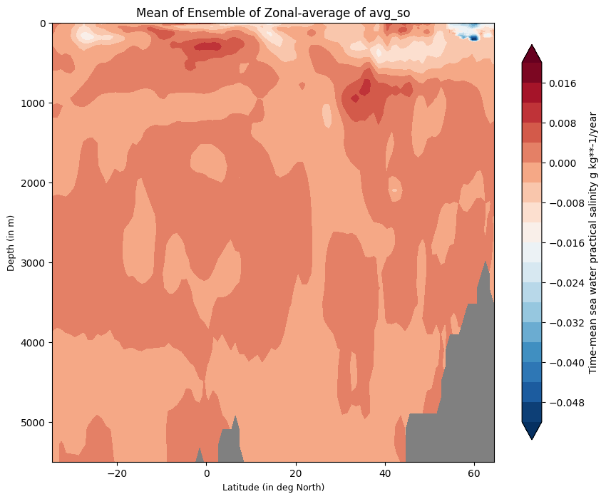
Ensemble-Zonal mean for average Time-mean sea water practical salinity for IFS-NEMO historical-1990.

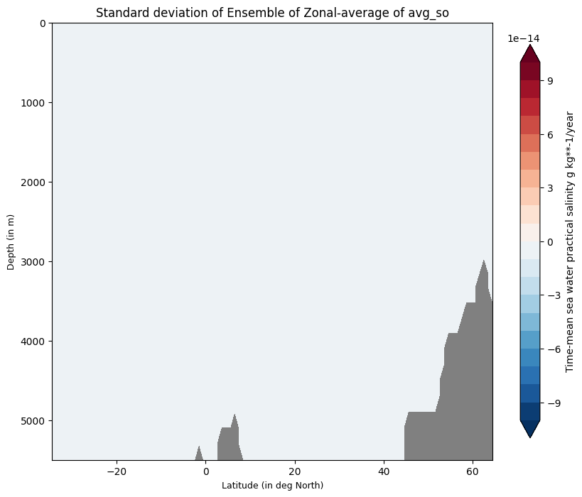
Ensemble-Zonal standard deviation for average Time-mean sea water practical salinity for IFS-NEMO historical-1990.

Available demo notebooks

Notebooks are stored in the notebooks/diagnostics/ensemble directory and contain usage examples.

• ensemble_zonalaverage.ipynb

Authors and contributors

This diagnostic is maintained by Maqsood Mubarak Rajput (@maqsoodrajput, maqsoodmubarak.rajput@awi.de). Contributions are welcome — please open an issue or a pull request. For questions or suggestions, contact the AQUA team or the maintainer.

Detailed API

This section provides a detailed reference for the Application Programming Interface (API) of the Ensemble Zonal diagnostic, produced from the diagnostic function docstrings.

Note

WORK IN PROGRESS